Static vs Dynamic Models in Drug Development: A Comprehensive Guide to Correlation Methods and Applications

Abstract

This article provides a comprehensive analysis of static and dynamic correlation methods essential for modern drug development. Tailored for researchers and pharmaceutical professionals, it explores the foundational principles of these modeling approaches, detailing their specific applications from early discovery to clinical risk assessment. The content delves into methodological execution, common challenges with optimization strategies, and rigorous validation frameworks. By synthesizing current research and comparative analyses, this guide serves as a critical resource for selecting the appropriate model to improve predictive accuracy, streamline development timelines, and enhance patient safety across therapeutic areas.

Core Principles: Understanding Static and Dynamic Modeling Fundamentals

Frequently Asked Questions (FAQs)

Q1: What is a mechanistic static model (MSM) in drug-drug interaction (DDI) prediction?

A mechanistic static model (MSM) is a mathematical tool used in early drug development to predict the risk of metabolic drug-drug interactions. It employs a set of equations to estimate the change in exposure (Area Under the Curve, or AUC) of a "victim" drug when co-administered with a "perpetrator" drug, based primarily on in vitro data. Unlike dynamic models, it uses fixed, or "static," surrogate driver concentrations for the perpetrator drug to represent its concentration at the enzyme interaction site (e.g., in the liver or gut) [1] [2]. Its primary purpose is for initial screening to flag potential interactions, ensuring patient safety by minimizing false-negative predictions [1].

Q2: When should I use a static model versus a dynamic PBPK model?

The choice between a static and a dynamic model depends on your development stage and the complexity of the question you need to answer. The following table outlines the primary applications and limitations of each approach.

Model Type	Primary Applications	Key Limitations
Mechanistic Static Model (MSM)	- Early-stage DDI risk screening [1]- Flagging even minor AUC deviations for safety [1]- Supporting regulatory filing for study waivers and label recommendations in some cases [2]	- Uses fixed driver concentrations, not time-variable levels [1]- Cannot evaluate complex scenarios (e.g., active metabolites, dose staggering, multiple perpetrators) [1]- Limited ability to assess inter-individual variability and vulnerable patient populations [1]
Dynamic PBPK Model	- Quantitative DDI predictions for regulatory submissions [1] [2]- Assessing DDI risk in specific populations (e.g., organ impairment, genetic polymorphisms) [1]- Complex scenario testing (dose staggering, enzyme-transporter interplay, time-dependence) [1] [2]	- Resource-intensive development and validation [2]- Requires considerable expertise and high-quality input data [2]

Q3: What are the key assumptions and limitations of static models?

Static models operate on several critical assumptions, which are also their primary limitations:

• Assumption of Fixed Driver Concentration: The model assumes that a single, static concentration (like [I] representing the maximum (Cmax) or average steady-state (Cavg,ss) concentration) can adequately represent the perpetrator's inhibitory effect over the entire dosing interval. This ignores the dynamic, time-varying nature of real drug concentrations [1].
• Linearity and Time-Invariance: The models typically assume that pharmacokinetic processes are linear and time-invariant, which may not hold for all drugs [1].
• Limited Scope: They are generally unsuitable for predicting interactions involving mechanisms like time-dependent inhibition, enzyme induction, or transporter-mediated interactions without significant modifications [1] [2].
• Vulnerable Patient Risk: Static models may underpredict the DDI risk in vulnerable patient populations, as they do not routinely incorporate physiological variability. One study found a high rate of discrepancy (IMDR >1.25) in 37.8% of simulations for a 'vulnerable patient' representative [1].

Q4: What is the most common cause of inaccurate predictions from static models?

The choice of driver concentration ([I]) for the perpetrator drug is a major source of variability and potential inaccuracy [1]. Regulatory guidelines often recommend using the maximum unbound hepatic inlet concentration to minimize false negatives [1]. However, some studies suggest that using the unbound average steady-state concentration (Cavg,ss) can sometimes lead to predictions more comparable to dynamic models [2]. The discrepancy between model predictions often stems from this fundamental choice, as the dynamic model uses time-variable concentrations that more accurately reflect the in vivo situation [1].

Troubleshooting Guides

Problem 1: My static model prediction shows a significant DDI risk, but a clinical study is not feasible. What are my options?

Solution: Consider developing a dynamic Physiologically Based Pharmacokinetic (PBPK) model to refine the risk assessment.

• Action 1: Verify Input Parameters. Double-check all input parameters for the static model, especially the fraction of victim drug metabolized by the affected enzyme (fm) and the inhibition constant (Ki) of the perpetrator. Ensure they are derived from robust and relevant in vitro studies.
• Action 2: Develop a PBPK Model. If resources allow, develop and qualify a PBPK model for both the victim and perpetrator drugs. This allows for a more quantitative prediction and can investigate "what-if" scenarios that static models cannot address [2].
• Action 3: Use a "Vulnerable Patient" Simulation. If a full PBPK model is not an option, use the static model with different driver concentrations (e.g., Cmax and Cavg,ss) to understand the range of possible outcomes. Be conservative in your interpretation, acknowledging that the risk for some patients may be higher than predicted [1].

Problem 2: I am getting different DDI predictions when using Cmax versus Cavg,ss as the driver concentration. Which one should I use?

Solution: The choice depends on the context and regulatory guidance.

• Step 1: Define the Objective. For initial screening and to avoid false negatives (i.e., missing a true DDI risk), the use of [I] = Cmax or the unbound maximum hepatic inlet concentration is recommended by regulatory guidelines [1].
• Step 2: Assess Consistency with Dynamic Models. Some research indicates that using [I] = Cavg,ss can yield predictions closer to those from dynamic PBPK models for certain applications [2]. If your goal is to compare directly with a PBPK simulation or for specific regulatory submissions where this approach has been accepted, Cavg,ss might be more appropriate.
• Step 3: Report the Range. A prudent practice is to calculate and report the DDI risk using both Cmax and Cavg,ss as a sensitivity analysis. This provides a range of possible outcomes and demonstrates a thorough understanding of the model's limitations.

Problem 3: How can I validate the predictions from my static model?

Solution: While static models are often used prospectively before clinical data is available, their predictions should be compared against observed data whenever possible.

• Methodology:
  • Conduct a Clinical DDI Study: This is the gold standard for validation. Compare the predicted AUC ratio (AUCr) from the static model with the observed AUCr from the clinical study.
  • Perform a Correlation Analysis: Plot the observed AUCr values against the predicted ones. Calculate the correlation coefficient and, more importantly, use statistical methods like Bland-Altman's limits of agreement to assess agreement, as the correlation coefficient alone can be misleading [3].
  • Evaluate Predictability: A common validation criterion is to check if the prediction error for the AUCr is within a pre-defined range (e.g., ±15-20%). If the static model consistently over- or under-predicts, it may indicate a systematic issue with the chosen driver concentration or other input parameters.

Experimental Protocols & Data

Core Equations for Competitive Inhibition MSM

The fundamental equation for predicting the AUC ratio (AUCr) for a victim drug in the presence of a competitive inhibitor is [1]:

AUCr = 1 / [ (Fg * Fh) ]

Where:

• Fg = 1 / [fg + (1 - fg) * (1 / (1 + ([I]_{gut} / K_i)) ) ] (Fraction escaping gut metabolism)
• Fh = 1 / [fh + (1 - fh) * (1 / (1 + ([I]_{liver} / K_i)) ) ] (Fraction escaping hepatic metabolism)
• [I]_{gut} and [I]_{liver} are the driver concentrations of the inhibitor at the gut and liver sites, respectively.
• K_i is the inhibition constant.
• fg is the fraction of the victim drug metabolized in the gut.
• fh is the fraction of the victim drug metabolized in the liver.

Quantitative Comparison of Static vs. Dynamic Models

A large-scale simulation study (2024) involving 30,000 simulated DDIs highlighted the discrepancies between static and dynamic models. The Inter-Model Discrepancy Ratio (IMDR) was defined as AUCr_dynamic / AUCr_static [1]. The table below summarizes the key findings on model discrepancy.

Simulation Scenario	Driver Concentration	Incidence of IMDR < 0.8 (Sponsor Risk)	Incidence of IMDR > 1.25 (Patient Risk)
'Population' Representative	Cavg,ss	85.9%	3.1%
'Vulnerable Patient' Representative	Not Specified	Not Specified	37.8%

Data adapted from [1]. IMDR outside 0.8-1.25 indicates a discrepancy.

Key Research Reagent Solutions

The following table lists essential "reagents" or tools required for building and applying mechanistic static models.

Item	Function in Experiment
In Vitro System (e.g., human liver microsomes, recombinant CYP enzymes)	To determine enzyme kinetic parameters for the victim drug (fm, Km, Vmax) and the inhibition constant (Ki) for the perpetrator drug [1].
Perpetrator Drug Pharmacokinetic Data	To calculate the static driver concentrations ([I]), such as unbound Cmax or unbound Cavg,ss [1] [2].
Victim Drug Pharmacokinetic Data	To understand the clearance mechanisms and the fraction of drug absorbed, which informs the Fg and Fh calculations [1].
Mechanistic Static Model Equations	The mathematical framework (see Core Equations above) that integrates in vitro and PK data to compute the predicted DDI magnitude (AUCr) [1] [2].
PBPK Software (e.g., Simcyp)	Used as a dynamic model comparator to evaluate the performance and potential bias of the static model predictions [1].

Workflow and Relationship Diagrams

Diagram 1: Static vs Dynamic Model Decision Workflow

Diagram 2: Key Components of a Static Model

Scientific FAQ: Core Principles and Applications

Q1: What fundamentally distinguishes a dynamic PBPK model from a simple static model?

A dynamic PBPK model is a time-dependent, mechanistic system that uses differential equations to simulate the concentration of a compound in various organs and tissues over time. It is structured based on real human physiology, incorporating anatomical (e.g., organ volumes) and physiological (e.g., blood flow rates) parameters. These models are multi-compartmental, with compartments representing specific organs like the liver or kidney, interconnected by the circulating blood or lymph system [4] [5] [6]. This allows for the prediction of full concentration-time profiles at the site of action, which may be difficult to measure experimentally [6] [7].

In contrast, a static model relies on steady-state assumptions and uses algebraic equations. While useful for predicting overall drug exposure or the magnitude of interactions like drug-drug interactions (DDIs), static models cannot predict the shape of a plasma concentration-time curve, time-varying changes, or distribution kinetics [8]. The key differentiator is that PBPK models offer a dynamic, physiological, and mechanistic framework for prediction and extrapolation, whereas static models provide a simpler, non-mechanistic snapshot [5] [8].

Q2: What are the primary assumptions when defining the structure of a PBPK model?

Two primary assumptions govern how drugs are distributed from blood into tissues [5] [7]:

• Perfusion-Rate Limited (Flow-Limited) Model: This assumes that tissue membranes present no barrier to diffusion. The rate-limiting step for a drug's distribution into a tissue is the rate of blood delivery to that tissue. This is typically true for small, lipophilic drugs. The model assumes that at steady state, the free (unbound) drug concentrations in the tissue and blood are equal [5].
• Permeability-Rate Limited (Membrane-Limited) Model: This applies when the permeability across the cell membrane is the rate-limiting step, often for larger or polar molecules. The tissue is conceptually divided into sub-compartments, such as intracellular and extracellular space, separated by a membrane that acts as a diffusional barrier [5].

Q3: In what key areas are dynamic PBPK models most critically applied in drug development?

PBPK modeling has become integral to regulatory submissions and drug development [6] [8] [7]. A systematic review of published models identified the most common applications as follows [8]:

Table 1: Primary Applications of PBPK Models in Drug Development

Application Area	Prevalence in Publications	Primary Utility
Drug-Drug Interaction (DDI) Predictions	28%	Predicting metabolic and transporter-mediated interactions to support dose adjustments and clinical trial design [8] [7].
Interindividual Variability & General PK Predictions	23%	Simulating population variability to understand exposure and response differences [8].
Formulation & Absorption Modeling	12%	Simulating the impact of drug properties and formulation on absorption kinetics, including food effects [8].
Predicting Age-Related PK Changes	10%	Extrapolating adult data to pediatric and geriatric populations via virtual simulations [6] [8].
Extrapolation to Diseased Populations	Not specified	Predicting pharmacokinetics in patients with hepatic or renal impairment by incorporating population-specific physiological changes [6].

Troubleshooting Guide: Computational Performance

Q1: Our PBPK model simulations are running slowly, especially for large-scale Monte Carlo analyses. What factors can we adjust to improve computational time?

Computational time is a critical consideration for analyses requiring hundreds of thousands of simulations [9]. Recent research has identified key factors that impact simulation speed.

Table 2: Factors Influencing PBPK Model Computational Time

Factor	Impact on Computational Time	Recommended Action
Model Compartment "Lumping"	High	Combine tissues with similar perfusion and lipid content (e.g., grouping slow-perfused tissues like muscle and skin) to reduce the number of state variables and differential equations. A 36% decrease in state variables led to a 20-35% reduction in computational time [9].
Treatment of Physiological Parameters	High	Treat body weight and dependent quantities (e.g., organ volumes, blood flows) as fixed constants rather than time-varying parameters. This can result in a ~30% time savings [9].
Implementation Platform	Medium	Using a compiled language (C, Fortran) is faster than interpreted languages (R, Python). A hybrid approach (e.g., using R with MCSim) balances ease-of-use and speed [9].
Number of Output Variables	Low	Decreasing the number of calculated output variables that are saved from the simulation has a minimal impact on core computational time [9].

Q2: We are using a flexible PBPK model template. Why might it be slower than a stand-alone implementation, and is this acceptable?

Yes, this is an expected trade-off. A general-purpose PBPK model template includes more compartments and options than are typically needed for any single chemical-specific model. During simulation, expressions for many unused quantities are still evaluated, which increases computational time compared to a lean, stand-alone model built for a single purpose [9]. The reduced human time required for model preparation and quality assurance review of a template-based implementation often justifies the increase in computational time [9].

Experimental Protocol: A Timing Experiment for PBPK Model Implementation

Objective: To quantitatively evaluate the impact of different model implementation decisions on the computational time required for PBPK model simulations.

Background: As PBPK models are used for more complex analyses (e.g., Monte Carlo simulations), understanding the drivers of computational speed is essential for efficient workflow [9]. This protocol outlines a method to systematically test these factors.

Materials and Reagents:

Table 3: Research Reagent Solutions for PBPK Timing Experiments

Item Name	Function/Description	Example Sources
PBPK Model Template	A pre-defined model "superstructure" with equations and logic for many PBPK features. Provides flexibility for testing different structures.	Bernstein et al. 2021/2023 [9]
Stand-Alone PBPK Model	A chemical-specific model implementation with a fixed, minimal structure. Serves as a performance benchmark.	U.S. EPA (2011) DCM model [9]
Simulation Software Platform	Software to execute the PBPK model and record simulation time.	R with MCSim, Simcyp, GastroPlus, PK-Sim [9] [7]
Chemical-Specific Parameters	Validated parameter sets for test compounds. Ensures comparisons are scientifically valid.	Dichloromethane (DCM) and Chloroform (CF) models [9]
Exposure Scenarios	Pre-defined exposure protocols to run consistent simulations.	Constant continuous oral, periodic inhalation, etc. [9]

Methodology:

• Model Configuration: Implement the chosen PBPK models (e.g., for DCM and CF) in both a template structure and a stand-alone structure [9].
• Factor Selection: Define the independent variables to test:
  • Compartment Number: Implement the model with and without "lumped" tissue compartments [9].
  • Parameter Type: Run simulations with body weight and dependent parameters set as both fixed constants and as time-varying quantities [9].
  • Output Detail: Configure the model to calculate a minimal vs. an extensive set of output variables [9].
• Simulation Execution: For each model configuration, run a set number of simulations (e.g., 1,000) for each of the four exposure scenarios. Ensure all simulations are performed on identical hardware.
• Data Collection: Precisely measure and record the computational time required for each set of simulations, excluding model loading and data-saving overhead.
• Data Analysis: Compare the average computational times across different configurations to quantify the impact of each factor.

This experimental approach directly enabled researchers to identify that fixing body weight parameters and reducing state variables significantly improves computational speed [9].

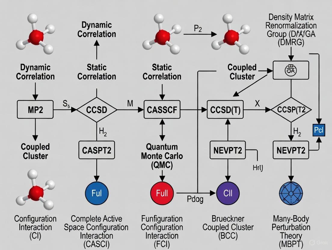
Conceptual Visualization: From Static to Dynamic Correlation in PK Modeling

The evolution from static to dynamic (PBPK) modeling represents a shift from empirical correlation to mechanistic, physiology-based simulation. The following diagram illustrates this conceptual and structural difference.

Frequently Asked Questions (FAQs)

1. What is electronic correlation, and why is it important in computational drug design? Electronic correlation is the interaction between electrons in the electronic structure of a quantum system. It is crucial because the Hartree-Fock (HF) method, a common starting point in computational chemistry, does not account for the instantaneous Coulomb repulsion between electrons, instead having each electron interact with the average field of all others. This missing interaction energy—the correlation energy—is vital for accurately predicting molecular properties, reaction pathways, and binding affinities, which are essential for rational drug design [10] [11] [12].

2. What is the fundamental difference between dynamic and static correlation? The fundamental difference lies in their physical origin and how they are addressed:

• Dynamic Correlation: Arises from the local, short-range repulsion between electrons that prevents them from coming too close to each other. It is related to the instantaneous dynamics of electron motion and can be recovered by adding a large number of electronic configurations (Slater determinants), each with a small weight, to the wavefunction [10] [11].
• Static (or Non-dynamic) Correlation: Occurs when a system's ground state cannot be qualitatively described by a single Slater determinant, often in cases with (near-)degeneracies, such as in bond-breaking or diradicals. It requires a linear combination of a few determinants with weights comparable to the HF determinant [10] [11] [12].

3. My calculations on a transition metal complex are qualitatively wrong. Could this be a static correlation issue? Yes, this is a classic symptom of significant static correlation. Transition metal complexes often have closely spaced electronic states (near-degeneracy). A single-determinant method like HF cannot properly describe this, leading to incorrect predictions. You should employ a multi-configurational method like MCSCF (Multi-Configurational Self-Consistent Field) to first capture the static correlation before applying dynamic correlation corrections [10] [12].

4. For a typical organic drug molecule, which type of correlation is more important? For most closed-shell, organic drug molecules near their equilibrium geometry, dynamic correlation is typically the dominant concern. The Hartree-Fock solution is often qualitatively correct, and the missing correlation energy can be recovered using methods like MP2 or CCSD(T) to achieve quantitative accuracy for properties like interaction energies and conformational barriers [10].

5. Can a method capture both dynamic and static correlation simultaneously? While some methods specialize in one type, it is nearly impossible to completely separate the two effects as they stem from the same physical interaction [10] [11]. High-level methods aim to capture both:

• Multi-Reference Methods: e.g., CASPT2 or MRCI, use an MCSCF reference (for static correlation) and then add perturbative or configurational corrections for dynamic correlation [12].
• Advanced Single-Reference Methods: At high orders, methods like CCSD(T) can incorporate some static effects, but may fail in cases of strong static correlation [10].

Troubleshooting Guides

Problem 1: Poor Description of Bond Dissociation

Symptoms: When calculating a potential energy surface, the energy becomes increasingly unrealistic as a bond is stretched. The dissociation products are incorrectly predicted.

Suspect Issue	Diagnostic Check	Recommended Solution
Strong Static Correlation	Perform a stability analysis on the HF wavefunction. Check for (near-)degeneracy of molecular orbitals involved in the bond.	Switch to a multi-configurational method (e.g., MCSCF/CASSCF). Select an active space that includes the bonding/antibonding orbital pair and relevant electrons.

Experimental Protocol: Diagnosing Static Correlation with CASSCF

• Geometry: Generate molecular structures along the reaction coordinate (e.g., varying bond length).
• Initial Calculation: Run a preliminary HF calculation to obtain molecular orbitals.
• Active Space Selection: This is critical. For a single bond dissociation, a minimal active space of 2 electrons in 2 orbitals (2e,2o) is a starting point.
• CASSCF Calculation: Perform a CASSCF calculation for each geometry, ensuring state-averaging if needed to describe degenerate states.
• Analysis: Plot the CASSCF potential energy curve. It should qualitatively correct the dissociative behavior. For quantitative results, dynamically correlate this wavefunction (e.g., with CASPT2).

Problem 2: Inaccurate Interaction Energies (e.g., Drug-Target Binding)

Symptoms: Binding or interaction energies are significantly over- or under-estimated, even after correcting for basis set superposition error (BSSE).

Suspect Issue	Diagnostic Check	Recommended Solution
Insufficient Dynamic Correlation	Compare the HF interaction energy with a higher-level method (e.g., MP2 or CCSD(T)) in a moderate basis set. A large discrepancy indicates strong dynamic correlation effects.	Use a method that accounts for dynamic correlation: MP2 (good for dispersion), CCSD(T) ("gold standard"), or DFT with empirical dispersion for larger systems. Ensure you use a sufficiently large basis set.

Experimental Protocol: Accurate Binding Energy Calculation using CCSD(T)

• System Preparation: Generate optimized geometries for the drug, target, and the drug-target complex.
• Basis Set Selection: Choose a correlation-consistent basis set (e.g., cc-pVDZ, aug-cc-pVDZ for weak interactions).
• Single-Point Energy Calculations:
  • Perform a HF calculation as a baseline.
  • Perform a CCSD(T) calculation at the same geometry and basis set.
• BSSE Correction: Perform a counterpoise correction to account for basis set superposition error.
• Energy Calculation: Binding Energy = E(complex) - E(drug) - E(target), using CCSD(T) energies and BSSE correction.

Problem 3: Unphysical Charge or Spin Densities in Diradicals/Metal Complexes

Symptoms: Computed spin densities are delocalized incorrectly, or charge distributions do not match experimental evidence.

Suspect Issue	Diagnostic Check	Recommended Solution
Static Correlation & Symmetry Breaking	Check for spatial or spin symmetry breaking in the HF solution (e.g., an unrestricted HF solution lower in energy than restricted). Examine the natural orbital occupation numbers from a correlated calculation; values significantly different from 2 or 0 indicate static correlation.	Use a multi-reference method (MCSCF) that can correctly describe the multi-configurational nature of the wavefunction. Ensure the active space is large enough to capture all essential correlation effects.

Key Data Tables

Table 1: Comparison of Dynamic vs. Static Correlation

Feature	Dynamic Correlation	Static Correlation
Physical Origin	Instantaneous Coulomb repulsion between electrons [10] [11]	Inability of a single determinant to describe (near-)degenerate states [10] [11]
Dominant in...	Closed-shell molecules near equilibrium geometry [10]	Bond dissociation, diradicals, transition metal complexes [10] [12]
Typical Wavefunction	Many determinants, each with small weight (e.g., CISD, CCSD) [10]	Few determinants, each with large weight (e.g., MCSCF) [10]
Primary Methods	MP2, CCSD(T), DFT [10] [11]	MCSCF, CASSCF [10] [12]
Impact on Energy	Quantitative correction [10]	Qualitative and quantitative correction [10]

Table 2: Method Selection Guide for Correlation Treatment

Method Category	Examples	Best for...	Key Limitations
Static (Non-dynamic)	MCSCF, CASSCF	Bond breaking, diradicals, multi-configurational states [12]	Choice of active space is critical and non-trivial; misses dynamic correlation [12]
Dynamic	MP2, CCSD(T), DFT	Closed-shell systems, dispersion interactions, quantitative energetics [10]	CCSD(T) is computationally expensive; MP2 can be poor for some systems; DFT's accuracy depends on functional [10]
Combined	CASPT2, MRCI	Systems requiring both static and dynamic correlation (e.g., spectroscopy) [12]	Computationally very demanding; complexity in setup [12]

The Scientist's Toolkit: Research Reagent Solutions

Item	Function in Electronic Structure Studies
Basis Sets	Sets of mathematical functions (e.g., Gaussian-type orbitals) used to construct molecular orbitals. The size and quality (e.g., cc-pVDZ, aug-cc-pVQZ) critically determine the accuracy of the calculation [12].
Pseudopotentials	Effective potentials used to replace the core electrons of atoms, significantly reducing computational cost for heavier elements while maintaining accuracy for valence electron properties.
Active Space (in MCSCF)	The selection of which electrons and orbitals to include in the multi-configurational treatment. This is the central "reagent" for tackling static correlation and requires careful chemical insight [12].
Quantum Chemistry Software	Platforms (e.g., Gaussian, GAMESS, ORCA, Molpro) that implement the algorithms for solving the electronic Schrödinger equation using various methods and basis sets.

Frequently Asked Questions (FAQs)

1. Why is IVIVE important in modern drug development? IVIVE is crucial because it uses in vitro data to predict in vivo outcomes, which helps streamline drug discovery, reduce development timelines by 30-50%, and lower preclinical testing costs. It supports the 3Rs principle (Replacement, Reduction, and Refinement) in toxicology by minimizing reliance on animal studies and enhances risk assessment for clinical progression [13] [14].

2. What are the main challenges associated with IVIVE predictions? A primary challenge is the systematic underestimation of in vivo clearance, often by a 3- to 10-fold factor. Furthermore, translating subtle, toxicologically relevant signals from in vitro systems and accurately predicting outcomes for diverse drug parameter spaces remain significant hurdles [14] [13] [1].

3. When should I use static versus dynamic IVIVE models? The choice depends on the context and required precision. Static models are simpler and use fixed input parameters (e.g., maximum inhibitor concentration), making them suitable for initial screening and rank-ordering compounds. However, they are not equivalent to dynamic models for quantitative predictions. Dynamic models (Physiologically Based Pharmacokinetic or PBPK) use time-variable concentrations and are essential for capturing inter-individual variability, investigating complex scenarios like multiple perpetrators, and providing accurate predictions for vulnerable patient populations or regulatory submissions [1].

4. Which types of compounds are most suitable for IVIVE studies? Compounds are most suitable when the liver is the primary clearance pathway, and their metabolism is minimally affected by transporter proteins. Ideal compounds have straightforward metabolic profiles, well-documented human pharmacokinetic (PK) data for validation, and demonstrate good stability and solubility for reliable testing [14].

Troubleshooting Guides

Problem 1: Systematic Underprediction of Hepatic Clearance

Issue: IVIVE predictions consistently and significantly underestimate the actual in vivo hepatic clearance value [14] [15].

Solution: Optimize the in vitro experimental system and refinement of calculation methods.

• Action 1: Refine the Metabolic Environment: Modify the in vitro system to better mimic the in vivo cytosol. Using a HEPES-KOH buffer system has been shown to improve performance [15].
• Action 2: Correct the Calculation Method: Incorporate the apparent volume of distribution (Vd) to refine the estimation of intrinsic hepatic clearance (CL_int) derived from the Michaelis-Menten equation. This addresses a previously overlooked source of error [15].
• Action 3: Apply a Correction Factor: Develop laboratory-specific linear regression correction equations based on a set of commercial compounds with established human PK data [14].

Problem 2: Failure to Capture Critical In Vivo Toxicity Pathways

Issue: The in vitro to in vivo translation misses subtle but toxicologically critical signals, such as the expression of Cytochrome P450 enzymes [13].

Solution: Integrate advanced AI frameworks to enhance the biological relevance of predictions.

• Action 1: Employ a Generative AI Framework: Implement a tool like AIVIVE, which uses a GAN (Generative Adversarial Network) as a base translator. This generator is trained on paired in vitro and in vivo transcriptomic data (e.g., from Open TG-GATEs) to create synthetic in vivo profiles [13].
• Action 2: Apply Local Optimization: Use local optimizers (AI models) to post-process the GAN output, specifically refining the predictions for low-signal, biologically relevant gene modules that are often missed. This enhances the accuracy of key pathways like bile secretion and steroid hormone biosynthesis [13].

Problem 3: Discrepancies Between Static and Dynamic Model Predictions

Issue: Static and dynamic model predictions show significant discrepancies, leading to potential patient or sponsor risk in evaluating drug-drug interactions (DDIs) [1].

Solution: Understand the limitations of static models and use dynamic models for quantitative predictions.

• Action 1: Identify High-Risk Parameter Spaces: Be cautious when the drug parameter spaces (for both victim and perpetrator) are at the edges of existing drug parameter space. Static models are most likely to fail here [1].
• Action 2: Use Dynamic Models for Vulnerable Populations: For compounds intended for use in populations with known variability (e.g., polymorphisms, organ dysfunction), rely on dynamic PBPK models. Static models show the highest rate of discrepancy (>1.25-fold) when simulating "vulnerable patient" representatives [1].
• Action 3: Validate Driver Concentrations: If using a static model, understand that using the average steady-state concentration (C_avg,ss) as the inhibitor driver can lead to a high rate of discrepancy (over 85% in some cases) compared to dynamic models. The maximum concentration (C_max) is a more conservative choice [1].

Table 1: Comparison of Static vs. Dynamic IVIVE Models for DDI Prediction

Feature	Static Model	Dynamic (PBPK) Model
Model Complexity	Simple equations	Complex, physiologically realistic
Input Concentration	Fixed (e.g., Cmax or Cavg,ss)	Time-variable
Inter-individual Variability	Not incorporated	Incorporated via virtual populations
Quantitative Prediction	Not equivalent to dynamic models; high discrepancy rates [1]	High-fidelity; regulatory standard for quantitative predictions [1]
Best Use Case	Initial screening, rank-ordering, flagging potential risks [1] [14]	Final quantitative risk assessment, special populations, complex DDI scenarios [1]
Reported Discrepancy (IMDR*)	Up to 85.9% for 'population' and 37.8% for 'vulnerable patient' using Cavg,ss [1]	Used as the reference for calculating discrepancy [1]

IMDR (Inter-Model Discrepancy Ratio) = AUCr_dynamic / AUCr_static

Table 2: Performance of Optimized IVIVE Methods

Method	Reported Underprediction Factor	Key Improvement
Standard IVIVE	3- to 10-fold [14]	Baseline
Well-Stirred Model (Optimized)	1.25-fold (hepatocyte assay) [14]	Advanced assay standardization and data analysis
Refined Hepatic Clearance Model	Reduced from 28.1 to ~70 mL/min/kg (vs. in vivo 73.9 mL/min/kg) [15]	Incorporation of Vd and a more cytosolic-like in vitro environment

Experimental Protocols

Protocol 1: AIVIVE Framework for Toxicogenomics Translation

This protocol uses AI to translate in vitro transcriptomic data to in vivo-like profiles [13].

1. Data Sourcing and Preprocessing:

• Source: Obtain rat liver in vitro and in vivo (single-dose) transcriptomic profiles from the Open TG-GATEs database.
• Normalization: Normalize the transcriptomic files using the robust multi-array average (RMA) method.
• Filtering: Annotate probes and filter for a toxicologically relevant gene set, such as the rat S1500+.
• Pairing: For each compound, create pairwise samples by matching in vitro and in vivo profiles based on compound, dose, and time. Split the data by compound into training (80%) and test (20%) sets.

2. AIVIVE Model Training:

• Architecture: Implement a GAN-based translator. The generator (a fully connected neural network with multiple hidden layers and LeakyReLU activation) takes the in vitro profile, experimental condition labels, and noise as input to generate a synthetic in vivo profile.
• Training: Train the generator-discriminator pair iteratively. Use a cycle-consistency loss to ensure the generated profiles retain biological relevance.

3. Local Optimization:

• Refinement: Apply multiple local optimizers (AI models) to the GAN's output. These optimizers specifically refine the values of low-signal, biologically relevant gene modules that the GAN might have missed.

4. Model Evaluation:

• Metrics: Evaluate the synthetic in vivo profiles using cosine similarity, root mean squared error (RMSE), and mean absolute percentage error (MAPE).
• Biological Validation: Compare differentially expressed genes (DEGs), enriched pathways (e.g., bile secretion, chemical carcinogenesis), and performance in downstream tasks like necrosis classification.

AIVIVE Workflow Diagram

Protocol 2: Optimizing Hepatic Clearance Prediction

This protocol details a method to reduce the systematic underprediction of hepatic clearance [15].

1. Experimental Setup:

• Target Drug: Select a model compound like Metoprolol.
• In Vitro Assay: Perform a microsomal stability assay. To better simulate in vivo conditions, provide a more cytosolic-like environment (e.g., using a HEPES-KOH buffer system).
• Ex Situ Model: Conduct experiments using an Isolated Perfused Rat Liver (IPRL) system.
• In Vivo Reference: Perform a pharmacokinetic study in rats to establish the true in vivo hepatic clearance value.

2. Data Integration and Model Refinement:

• Calculate Intrinsic Clearance: Determine the in vitro intrinsic clearance (CL_{int, in vitro}) from the microsomal assay using the Michaelis-Menten equation.
• Refine with Volume of Distribution: Incorporate the apparent volume of distribution (Vd) to correct the CL_{int, in vitro} calculation, addressing a key source of error.
• Select Hepatic Clearance Model: Use the Well-Stirred Model (WSM) and integrate findings from the IPRL and PK studies to identify the optimal liver drug metabolism-driving concentrations for the extrapolation.

3. IVIVE Calculation:

• Apply the refined CL_int and optimized model to predict the in vivo hepatic clearance. Compare the predicted value to the measured in vivo result to validate the improvement.

Hepatic Clearance Optimization

The Scientist's Toolkit: Research Reagent Solutions

Table 3: Essential Materials for IVIVE Experiments

Reagent / Material	Function in IVIVE Studies
Primary Hepatocytes (Human/Rat)	Gold-standard in vitro system for metabolism studies; used to measure intrinsic clearance and generate transcriptomic data [13] [14].
Liver Microsomes	Subcellular fraction containing CYP450 enzymes; used for high-throughput metabolic stability assays [14] [15].
HEPES-KOH Buffer	Buffer system used to create a more physiologically relevant, cytosolic-like environment in microsomal assays, improving prediction accuracy [15].
Open TG-GATEs Database	A comprehensive toxicogenomics database providing paired in vitro and in vivo transcriptomic and pathological data for model training and validation [13].
S1500+ Gene Set	A curated set of genes relevant to toxicity pathways; used to filter transcriptomic data, reducing noise and focusing analysis [13].
Well-Stirred Model	The simplest and most widely used mathematical model for predicting hepatic clearance from in vitro data [14] [15].

This technical support center provides troubleshooting guides and FAQs to help researchers, scientists, and drug development professionals navigate key FDA and ICH guidelines. The content is framed within the context of research on dynamic versus static correlation differentiation methods, which are crucial for establishing robust and predictive models in pharmaceutical development.

The International Council for Harmonisation (ICH) brings together regulators and the pharmaceutical industry to harmonize global drug development through consensus-based guidelines [16]. These guidelines provide a critical framework for the application of various scientific models—from nonclinical safety prediction to clinical trial design—ensuring that methodologies are sound, results are reliable, and patient safety is protected.

For research focusing on dynamic versus static correlation differentiation methods, understanding this regulatory landscape is paramount. Your models, which may differentiate between time-dependent (dynamic) and point-in-time (static) relationships in data, must be developed and validated within this structured yet flexible framework to gain regulatory acceptance.

The table below summarizes the core ICH guidelines relevant to the development and application of predictive models and correlation methods in drug development.

ICH Guideline	Focus Area	Key Principles & Relevance to Model Applications	Status & Date
E6(R3) - Good Clinical Practice [16]	Clinical Trial Design & Conduct	Promotes Quality by Design (QbD), Risk-Based Quality Management, and flexibility for innovative designs and technologies. Directly supports the use of novel endpoints derived from correlation models.	Final (September 2025)
M3(R2) - Nonclinical Safety Studies [17] [18]	Nonclinical to Clinical Transition	Defines nonclinical safety study requirements to support human clinical trials. Models that correlate nonclinical data with potential human outcomes must adhere to these standards.	Final (January 2010); Q&A (March 2013) [19]
M7(R2) - Assessment of DNA Reactive Impurities [20]	Impurity Risk Assessment	Provides a framework for (Q)SAR models and other methods to assess and control mutagenic impurities. Critical for applying predictive computational models in safety qualification.	Final (July 2023)
E20 - Adaptive Designs for Clinical Trials [21]	Adaptive Clinical Trial Designs	Outlines principles for trials that modify design based on interim data. Relies heavily on statistical models and pre-specified rules for dynamic adjustments, directly involving correlation methodologies.	Draft (September 2025)

Frequently Asked Questions (FAQs)

How does ICH E6(R3) support the use of novel correlation methods in clinical trials?

ICH E6(R3) modernizes the clinical trial framework to be more flexible and proportionate, which is ideal for integrating novel correlation methods [16] [22].

• Principle of Flexibility and Innovation: The guideline "incorporates flexible, risk-based approaches and embraces innovations in trial design, conduct, and technology" [16]. This means that if your research on dynamic correlation methods leads to a novel biomarker or a new digital endpoint, the regulatory pathway for its use in a trial is more clearly defined.
• Data Integrity and Governance: E6(R3) emphasizes stronger expectations for data governance, including "audit trails, metadata, traceability, and secure system validation" [22]. When generating and processing data for your models, you must ensure that the computerised systems used are validated and that the data lifecycle is fully traceable to withstand regulatory scrutiny.
• Risk-Based Approach: The guideline requires that oversight be focused on factors "Critical to Quality" (CtQ) [22]. When proposing a new model, you should perform a risk assessment that identifies how the model and its output impact participant safety and trial result reliability. Your monitoring plan should then be tailored to these risks.

What are the key considerations for validating predictive models under ICH M7(R2)?

ICH M7(R2) focuses on using models, primarily (Q)SAR systems, to predict the mutagenic potential of impurities without needing extensive laboratory testing for every compound [20].

• Model Validation and Applicability: The guideline aims to "harmonize the considerations for assessment and control of DNA reactive (mutagenic) impurities" [20]. A key troubleshooting point is ensuring the (Q)SAR model you are using is scientifically valid and applicable to the chemical space of your pharmaceutical compound. Using two complementary methodologies (one statistical and one expert rule-based) is a common industry standard to increase predictivity.
• Documentation and Justification: You must thoroughly document the models used, all input parameters, and the rationale for accepting or overriding any predictions. This creates a transparent and defensible scientific record for regulatory review.

Our research involves dynamic PK/PD modeling to transition from nonclinical to clinical studies. How does ICH M3(R2) guide this?

ICH M3(R2) provides the framework for determining the scope and duration of nonclinical safety studies needed to support human clinical trials [17] [18]. PK/PD models are central to this transition.

• Dose Selection Justification: The guideline emphasizes the importance of adequate nonclinical data to support the safe starting dose and dose escalation in humans [18]. Your dynamic PK/PD models, which correlate exposure and response over time across species, must be built upon robust nonclinical data from pharmacology, pharmacokinetic, and toxicology studies conducted according to M3(R2) standards.
• Troubleshooting Study Design: A common challenge is designing nonclinical studies that generate data suitable for building predictive models. The M3(R2) Q&A document is a valuable resource for clarifying complex issues in implementation [19]. Ensure your toxicology studies include sufficient time points and dose levels to capture the dynamic relationships essential for your models.

We are designing an adaptive trial using a biomarker model. What principles from ICH E20 must we follow?

ICH E20 provides principles for the use of adaptive designs in confirmatory clinical trials [21]. These designs often rely on models that correlate biomarker data with clinical outcomes.

• Pre-specification and Control of Bias: The draft guidance emphasizes that "principles that are critical for ensuring clinical trials produce reliable and interpretable results" [21]. A major troubleshooting area is the pre-specification of the adaptive plan. The model used to inform adaptations (e.g., a correlation model between biomarker response and patient outcome) and all decision rules must be documented in the trial protocol and statistical analysis plan before data are unblinded for the interim analysis. This is vital to protect trial integrity and minimize operational bias.
• Statistical Rigor: The models and algorithms driving the adaptation must be statistically sound. The type I error rate (false positive) must be controlled, and the analysis plan must account for the adaptive nature of the design.

Experimental Protocol: A Risk-Based Approach to Model Application

This protocol outlines a general methodology for developing and applying a predictive model within a clinical trial, aligning with ICH E6(R3) and E20 principles.

Objective: To develop and implement a model correlating a dynamic biomarker (e.g., daily digital sensor output) with a static clinical endpoint (e.g., 6-month survival) to guide patient enrichment in an adaptive trial.

Step 1: Model Building & Pre-specification (Pre-Trial)

• Gather historical data from previous studies (clinical and nonclinical).
• Develop the initial correlation model, clearly defining its mathematical form and inputs.
• Pre-specify the model's intended use in the trial protocol. Define the performance thresholds the model must meet (e.g., a specific correlation coefficient or predictive accuracy in a validation set) to be triggered for the adaptation.

Step 2: System & Process Validation

• Computer System Validation: If the model is implemented in software, follow FDA expectations for system validation, including audit trails and data security, as underscored in E6(R3) [22].
• Procedure Validation: Develop and train all research staff on the Standard Operating Procedure (SOP) for using the model, including data input formats and interpretation of outputs.

Step 3: In-Trial Execution & Monitoring

• Data Collection: Collect the dynamic biomarker data according to the pre-defined methods.
• Interim Analysis: At the pre-specified interim analysis point, an independent statistical center executes the pre-specified model on the unblinded data.
• Adaptation Decision: The model's output is used by the pre-chartered data monitoring committee to make a recommendation (e.g., to enrich the trial population based on biomarker status).

Step 4: Documentation & Reporting

• Maintain meticulous documentation of all steps, including raw data, model code/software, interim analysis results, and the rationale for all decisions. This creates a defensible audit trail for regulatory inspection.

The Scientist's Toolkit: Research Reagent Solutions

The table below lists key materials and tools essential for working within the regulatory framework for model applications.

Tool / Reagent	Function in Regulatory Science & Model Application
Validated (Q)SAR Software	Computational tool to predict the mutagenic potential of impurities as per ICH M7(R2); requires validation to ensure predictions are reliable [20].
PK/PD Modeling Software	Platform for building quantitative models that correlate pharmacokinetic (exposure) data with pharmacodynamic (response) data across time, critical for M3(R2) transitions and E20 adaptations.
Clinical Trial Management System (CTMS)	Centralized system for managing trial operations; must be validated to ensure data integrity as required by ICH E6(R3) for audit trails and data security [22].
Electronic Data Capture (EDC) System	System for collecting clinical trial data; requires validation to ensure the accuracy and reliability of data used in dynamic models and endpoint assessments [22].
Standardized Data Formats (e.g., CDISC)	Provides a common language for data submission; using standardized formats is a regulatory expectation and is critical for building models that integrate data from multiple sources.

Workflow Visualization: Risk-Based Model Application Pathway

The diagram below visualizes the logical workflow for applying a predictive model within a clinical trial, incorporating key risk-based and quality-focused principles from ICH E6(R3).

Logical Pathway for Nonclinical to Clinical Model Translation

This diagram outlines the key stages and decision points in applying nonclinical models to inform clinical trial design, as guided by ICH M3(R2) and related guidelines.

From Theory to Practice: Implementation in Drug Discovery and Development

Troubleshooting Guides

Guide 1: Addressing Poor Model Performance in Static vs. Dynamic Correlation Scenarios

Problem: Your DDI prediction model shows high accuracy for competitive inhibition but fails to generalize for mechanism-based inhibition scenarios.

Explanation: This often stems from treating all enzyme interactions with static correlation models, ignoring dynamic correlation patterns where relationships between variables change based on unobserved physiological states [23]. Competitive inhibition relies on concentration-dependent binding affinity, while mechanism-based inhibition involves irreversible enzyme complex formation [24] [25].

Solution: Implement a dynamic correlation analysis (DCA) to identify latent factors governing correlation changes between drug pairs.

• Step 1: Calculate Liquid Association Coefficient (LAC) scores for all drug pairs to identify those with dynamic correlation patterns [23].
• Step 2: Apply the DCA method to extract Dynamic Components (DCs) that represent underlying physiological states affecting correlation [23].
• Step 3: Integrate DCs as latent variables into your ensemble machine learning model, such as those used in DDI-CYP frameworks [26] [27].

Verification: Retrain your model with these dynamic components. Performance on mechanism-based inhibition test sets should improve by >15% accuracy [23] [28].

Guide 2: Handling Time-Discrepant Results in Induction vs. Inhibition Studies

Problem: Experimental results show delayed onset of enzyme induction effects compared to rapid inhibition, causing mismatches with model predictions.

Explanation: This discrepancy arises from fundamental mechanistic differences. Competitive inhibition occurs rapidly (hours) as it depends on perpetrator drug concentration, while induction requires new enzyme synthesis, causing a delayed effect (days to weeks) [29] [30]. Static models often fail to capture this temporal dimension.

Solution: Incorporate temporal parameters into your DDI prediction framework.

• For Induction Modeling:
  • Factor in the time required for gene transcription and translation (typically 24-72 hours).
  • Use time-dependent parameters that reflect enzyme synthesis rates (t½ ≈ 36 hours for CYP450) [25].
• For Inhibition Modeling:
  • Competitive inhibition: Model offset based on perpetrator drug half-life [25].
  • Mechanism-based inhibition: Model offset based on enzyme regeneration rate (3-5 days) [25].

Verification: Plot observed vs. predicted concentration-time profiles for known inducers (e.g., rifampin) and inhibitors (e.g., ketoconazole). The mean absolute error should decrease by >20% across the time series.

Frequently Asked Questions (FAQs)

FAQ 1: Why does our ensemble model perform well on CYP3A4 substrates but poorly on CYP2C9, even though both use similar machine learning architectures?

This indicates a limitation in your model's applicability domain and feature representation. CYP isoforms have distinct active site geometries and chemical preferences [24] [29]. The model may be overfitting to features predominant in CYP3A4 substrates. Retrain with isoform-specific features and validate the model's applicability domain by ensuring inference sets are structurally similar to training data [26] [27].

FAQ 2: How can we differentiate between competitive and mechanism-based inhibition using in silico methods?

The key distinction lies in reversibility and time dependency. Use these computational indicators:

• Competitive Inhibition: High predicted binding affinity to the enzyme's active site, reversible kinetics in molecular dynamics simulations, and concentration-dependent effects [24] [30].
• Mechanism-Based Inhibition: Prediction of metabolite formation that can covalently modify the enzyme, time-dependent inhibition (TDI) patterns in simulated kinetics, and irreversible binding confirmed by docking studies [24] [25].

FAQ 3: What are the critical differences between static and dynamic correlation methods in DDI prediction?

Static correlation assumes consistent relationships between molecular descriptors and DDI outcomes, while dynamic correlation accounts for how these relationships change with latent biological variables [23] [31].

Table: Static vs. Dynamic Correlation Comparison

Feature	Static Correlation Methods	Dynamic Correlation Methods
Underlying Assumption	Fixed relationships between variables	Relationships change with latent states (e.g., Z) [23]
Computational Load	Lower	Higher (requires scanning for latent factors)
Interpretability	More straightforward	More complex but biologically richer [23]
Best Suited For	Competitive inhibition, simple kinetics	Mechanism-based inhibition, complex temporal patterns

FAQ 4: Our deep learning model (DDINet) achieves high accuracy but lacks explainability for clinical translation. How can we improve interpretability?

Integrate an Adverse Outcome Pathway (AOP) framework alongside your deep learning model. This provides mechanistic explainability by visualizing each predicted P450 interaction, from molecular initiating event through to the clinical outcome [27]. Additionally, use attention heatmaps to identify which chemical features the model prioritizes, as demonstrated in DDINet implementations [28].

Table: Key Pharmacokinetic Parameters for DDI Prediction

Parameter	Competitive Inhibition	Mechanism-Based Inhibition	Enzyme Induction
Onset Time	Hours (follows perpetrator drug t½) [25]	May be delayed if metabolite-mediated [25]	Days to weeks (requires new enzyme synthesis) [30]
Offset Time	2-4 days (dependent on drug t½) [25]	3-5 days (dependent on enzyme regeneration t½) [25]	Weeks (dependent on enzyme degradation t½)
Effect on Km	Increase (decreased affinity) [24]	Irreversible reduction in active enzyme	Increased enzyme pool (effectively decreases [S]/Km)
Effect on CL	Decrease (CL[24]<="" td="" vmax="" ≈="">	Significant decrease	Increase
Typical AUC Change	2-5 fold increase [29]	5-20+ fold increase	Can decrease AUC by >50%

Table: Performance Metrics of Advanced DDI Prediction Models

Model Name/Type	Reported Accuracy	Strengths	Limitations
DDI-CYP (Ensemble)	85% [26] [27]	Incorporates P450 interaction predictions; improved explainability with AOP	Performance degrades with novel structures outside applicability domain
DDINet	95.42% [28]	High accuracy; mechanism-wise prediction (absorption, metabolism, etc.)	Complex architecture; requires significant computational resources
Liquid Association (LA)	N/A (screening method)	Detects dynamic correlations governed by latent factors [23]	Computationally intensive; interpretation can be challenging
R-xDH7-SCC15	WTMAD: 2.05 kcal/mol [31]	Excellent for electronic structure properties related to metabolism	Specialized for static/dynamic electronic correlation, not clinical DDI directly

Experimental Protocols

Protocol 1: Differentiating Competitive vs. Mechanism-Based Inhibition

Objective: Determine the inhibition mechanism of a new chemical entity (NCE) against CYP3A4.

Principle: Competitive inhibition is reversible and immediate, while mechanism-based inhibition is time-dependent and irreversible [24] [25].

Materials:

• Human liver microsomes (HLM) or recombinant CYP3A4
• Test compound (NCE)
• Specific CYP3A4 substrate (e.g., midazolam)
• NADPH regenerating system
• LC-MS/MS for metabolite quantification

Procedure:

• Pre-incubation Variation: Set up two sets of incubations.
  • Set A: Pre-incubate HLM + NCE + NADPH for 30 minutes.
  • Set B: No pre-incubation (HLM + NCE mixed immediately with substrate and NADPH).
• Reaction: After pre-incubation (Set A) or immediately (Set B), add substrate (midazolam) to initiate the reaction for a fixed time (e.g., 10 minutes).
• Termination & Analysis: Stop the reaction and quantify the metabolite (1'-hydroxymidazolam) using LC-MS/MS.
• Data Interpretation: A significantly greater reduction in metabolite formation in Set A (with pre-incubation) compared to Set B indicates time-dependent, mechanism-based inhibition. Similar inhibition in both sets suggests reversible (competitive) inhibition [25].

Protocol 2: Implementing a Dynamic Correlation Analysis (DCA) for DDI Prediction

Objective: Identify latent dynamic correlation signals in transcriptomic data that affect drug-metabolizing enzyme interactions.

Principle: The DCA method identifies Liquid Association Coefficients (LAC) to find gene pairs whose correlations are governed by unobserved variables (Z) [23].

Materials:

• Gene expression matrix (e.g., from a panel of human liver samples)
• DCA computational algorithm [23]

Procedure:

• Data Preprocessing: Standardize the gene expression matrix so all variables have a mean of zero and a standard deviation of one [23].
• LAC Calculation: For all pairs of genes (X, Y) in your matrix, compute the LAC score. A high LAC suggests their correlation is dynamically regulated by a hidden factor.
• Seed Selection: Rank gene pairs by LAC scores and select the top pairs most likely to be dynamically correlated.
• Extract Dynamic Components (DCs): Apply the DCA algorithm to the selected seed pairs to extract the latent Z variables (DCs) that govern the dynamic correlations.
• Integration with DDI Model: Use the extracted DCs as additional input features in your machine learning model (e.g., the DDI-CYP ensemble) to account for dynamic biological states [23] [27].

Signaling Pathways & Workflows

DDI Mechanism Workflow

DDI Prediction with Dynamic Correlation

Research Reagent Solutions

Table: Essential Computational Tools for Metabolic DDI Prediction

Tool/Reagent	Function/Description	Application in DDI Research
DDI-CYP Framework	An ensemble machine learning model that uses P450 interaction predictions and molecular structures [26] [27].	Predicts DDIs with ~85% accuracy; provides explainable predictions via Adverse Outcome Pathways.
DDINet Architecture	A deep sequential learning model (LSTM, GRU, Attention) for mechanism-wise DDI prediction [28].	Achieves high accuracy (95.42%); classifies DDIs by mechanisms like metabolism and excretion.
Liquid Association Coefficient (LAC)	A metric to identify pairs of variables whose correlation is dynamically regulated [23].	Screens gene/drug pairs to find those most likely influenced by hidden biological states.
Dynamic Correlation Analysis (DCA)	A method to extract latent signals (Dynamic Components) that govern dynamic correlations [23].	Uncovers unobserved physiological variables (Z) that affect drug interaction outcomes.
Adverse Outcome Pathway (AOP)	A framework for visualizing sequential events from molecular initiation to adverse outcome [27].	Increases model explainability by mapping predicted P450 interactions to clinical effects.
Molecular Fingerprints (FCFP6, ECFP6)	Numerical representations of molecular structure and properties [27].	Used as input features for machine learning models to represent drug molecules.

Frequently Asked Questions (FAQs)

Fundamental Concepts

Q1: What is the primary goal of ADMET prediction in lead optimization? The primary goal is to turn a biologically active but flawed "hit" compound into a viable drug candidate by systematically improving its properties. This involves enhancing potency and selectivity while fixing pharmacokinetic or safety problems [32]. The process aims to balance multiple parameters—such as solubility, metabolic stability, and reduced toxicity—simultaneously, as improving one property can often negatively impact another [32].

Q2: How do 'dynamic' and 'static' modeling approaches differ in ADMET prediction? This distinction generally applies to the methods used for analysis and correlation of data. In a broader computational context, static methods are insensitive to the temporal order of data points (e.g., classical QSAR, random forest models). In contrast, dynamic methods are sensitive to temporal sequence and can model causal relationships or time-dependent phenomena [33] [34]. For ADMET, this translates to using dynamic methods like physiologically based pharmacokinetic (PBPK) models that simulate drug disposition over time, versus static models that might predict a single, fixed outcome like a binary classification of solubility [35] [36].

Q3: What are the most common reasons for late-stage failure that ADMET prediction can mitigate? Late-stage attrition is often attributed to suboptimal pharmacokinetics (PK) and unforeseen toxicity [37]. Poor oral bioavailability (influenced by absorption and metabolism) and off-target effects (e.g., interaction with the hERG channel, which can affect heart function) are major contributors [32] [38]. Machine learning (ML)-driven ADMET prediction helps de-risk projects by identifying these issues early, before significant investment is made [37] [39].

Technical and Methodological Questions

Q4: What types of machine learning models are most effective for ADMET prediction? No single algorithm is universally best, but state-of-the-art methodologies include [37]:

• Graph Neural Networks (GNNs): Directly model molecular structure as graphs, effectively capturing structure-property relationships.
• Ensemble Learning: Combines multiple models to improve robustness and predictive accuracy.
• Multitask Models: Trained to predict several ADMET endpoints simultaneously, which can enhance generalizability by learning shared representations. While deep learning architectures are powerful, simpler methods like decision tree ensembles (e.g., Random Forest) can also perform very well, with data quality and molecular representation often mattering more than the algorithm itself [37] [38].

Q5: How can I define the applicability domain of my predictive model? A model's applicability domain defines the chemical space where its predictions are reliable. It can be assessed by comparing the similarity between the training data and the new compounds being predicted [38]. Methods to define this domain often use molecular descriptors or fingerprints. The OpenADMET initiative is generating high-quality, consistent datasets to help the community systematically develop and test such methods [38].

Q6: When should I use a global model versus a local (series-specific) model? The choice depends on data availability and project stage [38]:

• Global Models: Trained on diverse chemical structures. They are best for early-stage screening of large virtual libraries or when working on a new chemical series with limited internal data.
• Local Models: Trained on analogs from a specific chemical series. They can provide more accurate predictions for lead optimization within that series but require sufficient synthesized compounds for training. Systematic comparisons using high-quality data are ongoing to better guide this choice [38].

Troubleshooting Guides

Poor Model Performance and Generalization

Problem: My ADMET prediction model performs well on training data but poorly on new compound series.

Possible Cause	Diagnostic Steps	Solution
Data Quality Issues	Audit data sources for consistency. Check for high experimental variability between batches or sources.	Prioritize internal, high-quality data. Use datasets from initiatives like OpenADMET, which are generated consistently [38].
Incorrect Applicability Domain	Analyze the chemical similarity between your training set and the new compounds.	Retrain the model with more relevant data, or use a local model specific to your chemical series [38].
Overfitting	Check for a large performance gap between training and test set accuracy.	Simplify the model architecture, apply stronger regularization, or use ensemble methods to improve generalizability [37].

Inconsistent or Uninterpretable Results from Complex Models

Problem: My complex ML model (e.g., deep neural network) provides accurate predictions but is a "black box," making it hard to gain scientific insight or gain regulatory acceptance.

Possible Cause	Diagnostic Steps	Solution
Inherent Model Complexity	The model lacks transparency (e.g., difficulty understanding which structural features drove a prediction).	Implement Explainable AI (XAI) techniques to interpret predictions [37]. Alternatively, use hybrid approaches that combine established mechanistic models (e.g., PBPK) with interpretable ML components, making results more scientifically plausible [39].

Integrating Multimodal Data

Problem: I have various data types (e.g., in vitro assay results, structural biology data, omics data) but struggle to integrate them effectively into my predictive models.

Possible Cause	Diagnostic Steps	Solution
Data Silos and Formatting	Data exists in disparate, non-standardized formats.	Develop a unified data pipeline. Adopt multimodal data integration strategies that leverage modern ML frameworks to merge different data types, enhancing model robustness and clinical relevance [37]. Initiatives like OpenADMET combine high-throughput experimentation, structural biology, and ML, providing a blueprint for integration [38].

Quantitative Data for Method Comparison

Table 1: Key ADMET Parameters and Optimization Targets

Table summarizing critical properties to predict and optimize during lead optimization.

Property Category	Specific Parameters	Optimal Ranges / Targets	Common Prediction Methods
Absorption	Permeability (Caco-2, P-gp substrate), Solubility	High permeability, low efflux by P-gp, good solubility [37]	ML classifiers & regressors, PBPK [37] [39]
Distribution	Volume of Distribution (Vd), Plasma Protein Binding	Suitable Vd for target tissue, moderate to high PPB for long half-life [37]	QSAR, In vitro-in vivo extrapolation (IVIVE) [37]
Metabolism	Metabolic Stability (e.g., Clint), CYP Inhibition/Induction	Low clearance, minimal CYP inhibition to avoid drug-drug interactions [32] [37]	CYP activity assays, ML on structural alerts, QSAR
Excretion	Renal/Biliary Clearance	Balanced clearance pathways [37]	Physiologically-based models
Toxicity	hERG inhibition, Genotoxicity, Organ-specific toxicity	No activity against hERG; minimal off-target toxicity [32] [38]	In vitro assays (e.g., hERG), ML models, structural alerts

Table 2: Comparison of Machine Learning Algorithms for ADMET Prediction

Table outlining the performance characteristics of different ML approaches.

Algorithm Type	Typical Use Case in ADMET	Relative Interpretability	Data Efficiency	Key Advantages
Decision Tree Ensembles (RF, XGBoost)	Classification & regression for various endpoints (e.g., solubility, CYP inhibition)	Medium	High	Robust, handles diverse descriptors, good on smaller datasets [38]
Graph Neural Networks (GNNs)	Predicting activity directly from molecular structure	Low	Low to Medium	Learns features automatically; no need for manual descriptor calculation [37]
Support Vector Machines (SVM)	Classification tasks (e.g., toxic vs. non-toxic)	Low	Medium	Effective in high-dimensional spaces [40]
Multitask Learning Networks	Simultaneous prediction of multiple ADMET properties	Low	Medium	Improved data utilization; can enhance accuracy via shared learning [37]

Experimental Protocols

Protocol: Developing a Machine Learning Model for hERG Inhibition Prediction

Objective: To build a binary classification model that predicts the likelihood of a compound inhibiting the hERG channel.

Workflow Overview:

Materials:

• Dataset: Publicly available hERG inhibition data (e.g., ChEMBL) or internal high-throughput screening data.
• Software: Python/R with cheminformatics libraries (RDKit, OpenBabel).
• ML Libraries: Scikit-learn, XGBoost, Deep Graph Library (for GNNs).

Procedure:

• Data Collection: Curate a dataset of compounds with reliable hERG inhibition labels (e.g., IC50 < 10 µM = active). Note: Be aware of inter-assay variability; data from a single, consistent source is preferable [38].
• Data Curation: Standardize chemical structures (remove salts, neutralize charges), and handle duplicates and inaccurate entries.
• Molecular Featurization: Convert molecules into numerical representations.
  • Options: Extended-connectivity fingerprints (ECFPs), molecular descriptors (e.g., molecular weight, logP), or graph representations for GNNs.
• Model Training & Validation:
  • Split data into training (~70%), validation (~15%), and hold-out test sets (~15%).
  • Train multiple algorithms (e.g., Random Forest, XGBoost, Neural Networks).
  • Optimize hyperparameters using the validation set.
  • Evaluate final model performance on the hold-out test set using metrics like AUC-ROC, precision, and recall.
• Prospective Testing: Synthesize and test a set of novel compounds not used in training to validate the model's real-world predictive power [38].

Protocol: Implementing a PBPK Model for Human PK Prediction

Objective: To use a physiologically based pharmacokinetic (PBPK) model to simulate the absorption, distribution, and clearance of a lead compound in humans.

Workflow Overview:

Materials:

• Software: Commercial PBPK platform (e.g., GastroPlus, Simcyp) or open-source tool.
• Input Data: In vitro assay results (e.g., solubility, permeability, metabolic stability in human liver microsomes), physicochemical properties (logP, pKa), and protein binding data.

Procedure:

• Gather Input Parameters: Compile all necessary compound-specific physicochemical and in vitro data.
• Build and Verify Model: Populate the PBPK software with the compound parameters and select the appropriate human population model. Verify the model's plausibility.
• Simulate and Analyze: Run simulations to predict human PK profiles, including plasma concentration-time curves, C~max~, AUC, and half-life.
• Refine with Data: As clinical data becomes available (e.g., from Phase I trials), refine the model by adjusting parameters within physiological bounds to improve its predictive accuracy for subsequent simulations [35] [36].

The Scientist's Toolkit: Research Reagent Solutions

Tool / Resource	Type	Primary Function	Example Use Case
RDKit	Software Library	Cheminformatics and ML	Generating molecular fingerprints and descriptors for QSAR models [40].
SwissADME	Web Tool	ADME Prediction	Rapid, free prediction of key properties like logP, solubility, and CYP inhibition [32].
PBPK Platforms (e.g., Simcyp, GastroPlus)	Software	Mechanistic PK Modeling	Predicting human pharmacokinetics and drug-drug interactions from in vitro data [39] [35].
OpenADMET Data	Data Resource	High-quality experimental data	Training and validating ML models on consistent, reliable datasets [38].
CACO-2 Assay Kit	In Vitro Assay	Measuring Intestinal Permeability	Experimental determination of a compound's absorption potential [37].
hERG Inhibition Assay	In Vitro Assay	Cardiac Safety Screening	Experimentally testing a compound's potential for hERG channel blockade [38].

Dose Regimen Selection and First-in-Human (FIH) Dose Prediction

Frequently Asked Questions (FAQs)

FAQ 1: Why is the traditional Maximum Tolerated Dose (MTD) approach no longer sufficient for modern oncology drugs?

The traditional MTD approach, often determined via a '3+3' trial design, focuses primarily on short-term safety and dose-limiting toxicities [41] [42]. While this was suitable for cytotoxic chemotherapies, it is less ideal for targeted therapies and immunotherapies. Studies show that nearly 50% of patients on targeted therapies in late-stage trials require dose reductions, and the FDA has required post-approval dosing re-evaluation for over 50% of recently approved cancer drugs [42]. This is because the MTD approach often selects unnecessarily high doses that increase toxicity without providing additional efficacy, a key issue given that modern drugs often have a flatter exposure-response relationship [41] [43].

FAQ 2: What are the key differences between static and dynamic correlation methods in dose-response analysis?

Static correlation methods, like Pearson's correlation, are insensitive to the temporal order of data points and provide a single, averaged measure of association. In contrast, dynamic correlation methods, such as lagged-cross-correlation (LCC) or autoregressive models, are sensitive to temporal precedence and can model how relationships evolve over time [34] [33]. In drug development, this translates to using dynamic models to understand how drug exposure over time (pharmacokinetics) dynamically influences efficacy and safety outcomes (pharmacodynamics), which is crucial for identifying the optimal biological dose rather than just the maximum tolerated one [41] [34].

FAQ 3: What model-informed approaches are recommended for FIH dose selection?

Model-informed drug development (MIDD) approaches are critical for FIH dose prediction. Key methods include:

• Quantitative Systems Pharmacology (QSP) Models: These mechanistic models incorporate biological mechanisms and drug properties to simulate human pharmacology and predict dose-response, helping to de-risk FIH decisions [41] [44].
• Population PK/PD Modeling: This correlates or links changes in drug exposure to changes in clinical endpoints (safety or efficacy) and can account for confounding factors like concomitant therapies [41].
• Exposure-Response Modeling: This uses nonclinical and early clinical data to predict the probability of efficacy and adverse reactions as a function of drug exposure, helping to simulate the benefit-risk profile of different dosing regimens [41].

FAQ 4: How can I select doses for further exploration after the FIH trial?

Selecting doses for proof-of-concept trials requires a fit-for-purpose approach that leverages all available data [42]. Strategies include:

• Backfill and Expansion Cohorts: Increasing the number of patients at specific dose levels within early-stage trials to strengthen the understanding of the benefit-risk ratio [42].
• Biomarker Integration: Using biomarkers like circulating tumor DNA (ctDNA) levels can help identify therapeutic responses that may not be detected with short-term follow-up [42].
• Clinical Utility Indices (CUI): Providing a quantitative framework to collaboratively integrate diverse data types (e.g., efficacy, safety, PK/PD) to determine the most promising doses for further study [42].

Troubleshooting Common Experimental Challenges

Problem: Inability to differentiate direct drug effects from indirect or confounded effects in exposure-response analysis.

Solution: Employ dynamic, model-based methods that can account for temporal relationships and network effects.

• Recommended Protocol (Lagged-Cross-Correlation Analysis):
  • Data Preparation: Collect high-frequency, time-series data on drug exposure metrics (e.g., concentration) and response biomarkers [34] [45].
  • Feature Generation: Create lagged features (e.g., 6-hour, 12-hour lag) and rolling features (e.g., 24-hour average) from the time-series data to capture dynamic relationships [45] [46].
  • Model Application: Apply a lagged-cross-correlation (LCC) algorithm. In sparse, non-linear systems with delays, LCC has been shown to provide a reliable estimation of directed effective connectivity [34].
  • Validation: Compare the reconstructed connectivity (dose-effect relationship) against known ground truth if available, or use forward simulation to see if the estimated model can recreate the observed activity patterns [34].

Problem: High rate of dose modifications (reductions, interruptions) in late-stage trials due to intolerable side effects.

Solution: Shift from an MTD paradigm to an optimization paradigm that balances efficacy and safety early in development.

• Recommended Protocol (Exposure-Response & Safety Modeling):
  • Data Collection: Systematically collect landmark safety data (incidence of interruptions, reductions, discontinuations, specific adverse events) and preliminary efficacy data (e.g., overall response rate) across all dose levels in early trials [41].
  • Model Building: Perform a logistic regression analysis or population PK/PD modeling of key safety endpoints as a function of drug exposure (e.g., trough concentration, area under the curve) [41].
  • Simulation: Use the model to simulate the probability of severe adverse reactions and efficacy for various dosing regimens [41].
  • Dose Selection: Select the dosage for the registrational trial that balances a high probability of therapeutic response with an acceptable, lower probability of adverse reactions, potentially below the MTD [41] [43].

Table 1: Key Dosage Optimization Definitions and Metrics

Term	Definition	Application in Drug Development
Maximum Tolerated Dose (MTD)	The highest dose not causing unacceptable toxicity in a small cohort over a short duration [41] [42].	Traditional endpoint of dose-escalation; often the Recommended Phase 2 Dose (RP2D) for chemotherapies.
Minimum Effective Dose (MED)	The lowest dose that provides a clinically meaningful therapeutic benefit [43].	Aims to minimize toxicity while maintaining efficacy.
Optimal Biological Dose (OBD)	The dose that provides the best balance between efficacy and safety/tolerability [43].	Target for modern targeted therapies and immunotherapies.
Minimal Immunologically Active Dose (MIAD)	The lowest dose that triggers a meaningful immune response (relevant for immunotherapies) [43].	Used in immuno-oncology development to find a dose that engages the immune system without over-activation.

Table 2: Performance of Model-Informed Approaches vs. Traditional Methods

Method	Key Strength	Limitation	Context of Superior Performance
Lagged-Cross-Correlation (LCC) [34]	Reliably estimates directed connectivity in sparse, non-linear networks with delays; computationally simple.	Performance decreases in larger, less sparse networks; struggles without time delays.	Sparse, noise-driven systems with temporal delays.
Derivative-Based Methods (e.g., DDC) [34]	Good performance in linear systems or systems without time delays; high noise tolerance.	Assumes no time delays; may be less reliable in delayed, non-linear systems.	Linear networks or systems without spatio-temporal delays.
3+3 Dose Escalation [42]	Simple, widely understood design.	Poor at identifying true MTD; ignores efficacy and long-term tolerability.	Largely considered outdated for modern targeted therapies.
Model-Informed FIH (QSP) [44]	End-to-end solution; uses preclinical data to predict human dose-response; reduces errors via standardized workflows.	Requires robust preclinical data and model calibration.	All stages, from preclinical translation to clinical dose prediction.

Experimental Protocols

Protocol 1: Utilizing a QSP Workflow for FIH Dose Prediction

This protocol outlines a model-informed approach to select FIH doses using Quantitative Systems Pharmacology [44].

• Input Preclinical Data: Collect raw data from preclinical studies, including in vitro and in vivo PK, PD, target engagement, and efficacy data (e.g., tumor growth inhibition) [41] [44].
• Model Calibration: Calibrate the QSP model using the preclinical data. The model should incorporate known biology of the target and disease pathway.
• Human Simulation: Use the calibrated model to simulate human pharmacology. Simulate various dosing regimens and schedules to predict human PK and PD profiles.
• Target Exposure Identification: Define an efficacious target exposure (e.g., a target trough concentration) based on nonclinical efficacy models and knowledge of the target [41].
• Dose Projection: Run simulations to identify the dosing regimen in humans that is predicted to achieve the target exposure in >90% of patients throughout all treatment cycles [41] [44].
• Report Generation: Automatically output figures, tables, and a report detailing the projected FIH dose, the rationale, and the associated predictions for efficacy and safety [44].

Protocol 2: Implementing a Clinical Utility Index (CUI) for Dose Selection

This protocol is used after initial FIH data is available to quantitatively compare multiple doses and select the best candidate(s) for further study [42].

• Define Criteria: Identify key criteria for dose evaluation. These typically include measures of Efficacy (e.g., ORR, biomarker response), Safety (e.g., rate of Grade 3+ AEs, dose modifications), and Pharmacology (e.g., trough concentration, target occupancy) [41] [42].
• Assign Weights: Collaboratively assign a weight to each criterion based on its relative importance to the overall benefit-risk profile.
• Score Each Dose: For each dose level under consideration, assign a score for every criterion based on the collected clinical data.
• Calculate CUI: Compute the CUI for each dose as the weighted sum of its scores across all criteria. The formula is: CUI = (Weight_Efficacy * Score_Efficacy) + (Weight_Safety * Score_Safety) + ...
• Rank and Select: Rank the doses based on their final CUI score. The dose with the highest CUI represents the one with the most favorable overall profile and should be advanced to subsequent trials [42].

Research Reagent Solutions

Table 3: Essential Tools for Dose Optimization and Correlation Analysis

Tool / Reagent	Function / Explanation	Application in Research
QSP Modeling Platform (e.g., Certara IQ) [44]	A software platform providing pre-written code templates and optimized solvers for mechanistic QSP modeling.	Streamlines FIH dose prediction by simulating human pharmacology and dose-response from preclinical data.
Clinical Utility Index (CUI) [42]	A quantitative framework that serves as a "reagent" for decision-making, integrating multiple data types into a single score.	Objectively compares and ranks different dosing regimens based on a weighted combination of efficacy, safety, and PK/PD data.
Wearable Device (WD) Data [45] [46]	Provides continuous, objective physiological and activity data (e.g., heart rate, sleep, activity) as time-series inputs.	Used to generate lag and rolling features for predictive models of patient behavior, such as medication adherence, which can influence dose regimen feasibility.
Lagged-Cross-Correlation (LCC) Algorithm [34]	A computational method to estimate directed, effective connectivity by analyzing time-lagged correlations between variables.	Infers causal relationships in dose-response data, helping to differentiate direct drug effects from indirect effects in complex biological networks.

Signaling Pathways and Workflow Diagrams

Model-Informed FIH Dose Prediction Workflow

Static vs Dynamic Correlation Analysis Workflow

Frequently Asked Questions (FAQs)

1. What is the core difference between static and dynamic correlation methods in the context of organ aging research?

Static correlation methods, like Pearson's correlation, measure the overall statistical association between variables without considering the temporal order of data points. In contrast, dynamic correlation methods, such as lagged-cross-correlation (LCC) or multivariate autoregressive (AR) models, are sensitive to the sequence of time points and can infer the directionality of influence, which is crucial for understanding causal pathways in aging [33] [34]. In practice, for fMRI data, static and dynamic functional connectivity estimates often capture highly similar information, though dynamic methods may provide complementary insights in sparse, noise-driven systems with temporal delays [33] [34].

2. How can I validate that my organ-age prediction model is capturing biologically meaningful aging and not just chronological age?

A key validation is to demonstrate that the "age gap" – the difference between predicted biological age and chronological age – meaningfully predicts future health outcomes. For instance, individuals with a positive age gap (biologically older) should have a higher subsequent risk of organ-specific diseases and mortality, even after adjusting for chronological age. Research on proteomic aging clocks has shown that an accelerated brain age gap is strongly associated with future risk of neurodegenerative diseases, and all organ age gaps predict all-cause mortality [47]. Furthermore, your model should show that genetic variants associated with this age gap are linked to known age-related pathways and diseases [48].

3. What are the primary sources of confounding when building genetic association studies for biological age, and how can I control for them?

The main sources of confounding in such observational studies are:

• Selection Bias: Systematic differences in characteristics between your exposed and unexposed groups [49].
• Confounding by Indication: Sicker patients are both more likely to have certain physiological measures and more likely to have adverse outcomes [49].
• Population Stratification: Systematic differences in allele frequencies between subpopulations due to non-genetic reasons [48].

To control for these, you can use:

• Matching: Select subjects with similar characteristics (e.g., using propensity scores) to ensure comparability [49].
• Stratification: Analyze data within subgroups based on characteristics like sex, as aging dynamics can differ significantly between males and females [50].
• Modelling: Use statistical models like linear regression to adjust for known confounders such as age, sex, and genetic principal components [48] [49]. For genetic studies, using tools like LD score regression can help assess and correct for genomic inflation [48].

4. My model performs well in my primary cohort but fails in an external population. What could be the reason?

This often stems from a lack of generalizability. Common causes include:

• Cohort-Specific Social Norms: Your model may be relying on traits that reflect societal changes over time (e.g., "lifetime number of sexual partners") rather than pure biological aging. Always prioritize purely biological and physiological parameters [50].
• Limited Demographic Representation: Your training data may not encompass the genetic and environmental diversity of the target population. Models trained on European ancestry cohorts, like the UK Biobank, need validation in diverse ethnic groups [48] [47].
• Organ Aging Heterogeneity: The pattern of aging across different organs can vary between populations. Ensure your model accounts for the weak correlations between age gaps of different organ systems [47].

Troubleshooting Guides

Problem 1: Poor Generalization of Dynamic Correlation Estimates

Symptoms: Your dynamic connectivity model (e.g., lagged correlation, multivariate AR) fails to provide new information beyond static correlation or performs poorly when applied to new data.

Possible Cause	Solution
HRF Confounding: The hemodynamic response function (HRF) in fMRI blurs the neural signal, compromising the accurate estimation of temporal precedence and directionality [33].	Consider using HRF deconvolution techniques as a preprocessing step. Alternatively, validate your findings with neurophysiological data that is not affected by HRF, such as EEG/MEG [33].
Network Size and Sparsity: Dynamic methods like LCC work best for small, sparse networks. Performance decreases in larger, denser networks [34].	Assess if your network model's size and sparsity match the method's optimal use case. For larger networks, consider alternative approaches or ensure robust cross-validation [34].
Signal Stationarity: Your model assumes non-stationarity, but the underlying brain signals are largely stationary, meaning their statistical properties do not change over time [33].	Test the stationarity of your time series using methods like AR randomization. If stationarity cannot be rejected, a simpler static model may be sufficient and more reliable [33].

Problem 2: Integrating Genetic and Organ-Function Data is Statistically Underpowered

Symptoms: You are unable to detect significant genetic loci associated with organ age gaps, or your results are unstable.

Solution: Adopt a multiorgan framework to boost power and biological insight.

• Action 1: Perform a Multiorgan GWAS. Instead of focusing on a single organ, conduct a genome-wide association study (GWAS) across multiple organ systems simultaneously. This allows you to identify genetic variants with pleiotropic effects (affecting multiple organs) and those with organ-specific effects [48].
• Action 2: Establish Causal Networks. Use methods like two-sample Mendelian randomization to establish potential causal relationships between chronic diseases, lifestyle factors, and multiple organ age gaps. This creates a more powerful and interpretable multiorgan causal network [48].
• Example Workflow: A study on 377,028 UK Biobank participants identified 393 genomic loci associated with nine organ age gaps. They found that genetic variants were predominantly organ-specific but also revealed interorgan cross-talk, providing a systems-level view of aging genetics [48].

Problem 3: Choosing the Right Physiological Traits for an Organ Aging Clock

Symptoms: Your biological age prediction model is inaccurate or reflects societal trends rather than biology.

Solution: Implement a rigorous, biology-driven trait selection process.

• Action 1: Apply Strict Filtering Criteria. When selecting traits from a large dataset (e.g., UK Biobank), filter parameters based on three criteria [50]:
  • The trait should not reflect societal norms or structures.
  • The trait should not be a function of elapsed time.
  • The trait's value should not be computed using a person's chronological age.
• Action 2: Optimize for Organ System Coverage. A model that heavily weights traits querying multiple organ systems (lung, heart, brain, etc.) predicts chronological age most accurately and is likely a better measure of global biological aging. Do not rely on a single organ system [50].
• Action 3: Develop Parsimonious Models. For clinical translation, identify a minimal set of key physiological traits that retain strong predictive performance. One study successfully reduced a 121-trait model down to 12 key traits for a practical aging assessment [50]. Similarly, proteomic clocks can be built with a reduced panel of proteins (e.g., as few as 5 for heart aging) without sacrificing accuracy [47].

Key Experimental Protocols

Protocol 1: Building a Proteomic Organ Aging Clock

This protocol outlines the steps for creating a biologically interpretable, organ-specific aging model from plasma proteomics data, as demonstrated in recent research [47].

• Protein Selection & Cohort Split:

  • Identify organ-enriched proteins using tissue-level expression data from resources like the Genotype-Tissue Expression (GTEx) project.
  • Randomly split your cohort (e.g., UK Biobank) into a training set (e.g., 70%) and a test set (e.g., 30%).

• Model Training:

  • In the training set, use a nonlinear machine learning method, such as Light Gradient Boosting Machine (LightGBM).
  • Apply a feature selection algorithm (e.g., Boruta) to identify the subset of organ-enriched proteins that are most predictive of chronological age.
  • Train one model for each organ system using its respective organ-enriched proteins.

• Model Validation & Aging Phenotype Calculation:

  • Apply the trained models to the test set and external validation cohorts to assess prediction accuracy (correlation between predicted and chronological age).
  • For each individual and organ, calculate the organ age gap: the residual from regressing the proteomic-predicted age on chronological age. A positive gap indicates accelerated aging.

• Outcome Association:

  • Use Cox proportional hazards models to test if the organ age gap predicts the future onset of organ-specific diseases and all-cause mortality, adjusting for chronological age, sex, and other risk factors.

Protocol 2: Differentiating Static vs. Dynamic Functional Connectivity

This protocol provides a systematic framework for comparing correlation-based methods, suitable for analyzing neural or other physiological time-series data [33] [34].

• Method Selection: Choose representative methods from four key classes based on their sensitivity to temporal order and the number of variables considered. The table below summarizes this framework:

  Comparison Framework for Functional Connectivity Methods [33]

	Bivariate (Pairwise)	Multivariate (Network-wide)
Static (time-insensitive)	Pearson's Correlation	Partial Correlation
Dynamic (time-sensitive)	Lagged-Cross-Correlation (LCC)	Multivariate AR model (with/without self-connections)

• Similarity Assessment: Calculate the similarity between the connectivity matrices produced by the different methods. This can be done by correlating the matrices or comparing node-level centrality measures.

• Brain-Behavior Association Comparison: Test how well each connectivity estimate predicts a behavioral or physiological variable of interest (e.g., cognitive scores). Compare the patterns and strength of these associations across methods.

• Performance Validation (if ground truth is known): In simulated data with a known ground-truth connectivity matrix, evaluate which method most accurately reconstructs it. Research suggests that for sparse, non-linear networks with delays, a combination of LCC and derivative-based methods can be highly effective [34].

Research Reagent Solutions

Essential Materials for Organ Aging and Connectivity Research

Item	Function / Application
UK Biobank (UKB) Dataset	A large-scale biomedical database containing genetic, lifestyle, proteomic, and health information from ~500,000 participants. It is a primary resource for developing and testing aging models and genetic associations [48] [50] [47].
Olink Explore 3072 Panel	A high-throughput immunoassay platform for measuring 2,916 plasma proteins. Used to build proteomic aging clocks by quantifying organ-enriched proteins in large cohorts [47].
Genotype-Tissue Expression (GTEx) Database	A public resource containing tissue-specific gene expression data. Used to identify and select proteins that are enriched in specific organs for building organ-specific aging models [47].
Light Gradient Boosting Machine (LightGBM)	A fast, distributed, high-performance gradient boosting framework used for machine learning tasks like classification and regression. Ideal for training accurate aging prediction models on large datasets [47].
FUMA (FUctional Mapping and Annotation)	An online platform for the functional annotation of GWAS results. It helps to identify independent genetic signals and annotate their potential functional consequences, crucial for post-GWAS analysis [48].

Methodological Pathway and Experimental Workflow Diagrams

Research Workflow for Special Population Simulations

Controlling for Confounding in Observational Studies

Integration with AI and Machine Learning for Enhanced Predictions

This technical support center provides troubleshooting guides and FAQs for researchers, scientists, and drug development professionals working with AI and Machine Learning (ML) for enhanced predictions. The content is framed within the context of a broader thesis on dynamic versus static correlation differentiation methods research, focusing on practical experimental issues and their solutions.

Table 1: Global AI and ML in Drug Development Market Snapshot (2024-2034) [51]

Category	Specific Segment	Market Share or CAGR
Phase of Drug Development	Drug Discovery Segment (2024)	42% revenue share
	Clinical Trials Segment (Forecast)	29% CAGR
Technology Type	Machine Learning (Supervised/Unsupervised) (2024)	45% market share
	Generative AI & Foundation Models (Forecast)	35% CAGR
Function/Application	Target Identification & Validation (2024)	27% revenue share
	Drug Repurposing (Forecast)	31% CAGR
Therapeutic Area	Oncology (2024)	36% revenue share
	Metabolic Disorders (Forecast)	26% CAGR

Table 2: Performance Comparison of Connectivity Estimation Methods in Neural Networks [34] [52]

Method Type	Specific Method	Best Application Context	Key Performance Characteristics
Correlation-Based	Lagged-Cross-Correlation (LCC)	Sparse, non-linear networks with time delays [34] [52]	Most reliable estimation of ground truth connectivity in its context; lower computational cost vs. transfer entropy [34] [52].
Derivative-Based	Dynamic Differential Covariance (DDC)	Linear networks or systems without time delays [34] [52]	Reliably estimates directionality, high noise tolerance, good for non-stationary data [34].
Hybrid	LCC combined with derivative-based covariance	Sparse non-linear networks with delays [34] [52]	Provides the most reliable estimation of the known ground truth connectivity matrix [34] [52].

Troubleshooting Guide: FAQs for AI/ML Experiments

FAQ 1: My AI model is technically sound but fails to have any business or research impact. What is the root cause?

This is a classic symptom of a disconnect between the ML team and the business or research domain [53]. The solution is to foster enhanced interdisciplinary collaboration [54].

• Root Cause: ML teams often work in isolation, building solutions for poorly defined or low-priority problems without deep domain expert input [53]. This leads to a misalignment between the model's objectives and the core research goals.
• Solution:
  • Establish Cross-Functional Teams: Create teams that blend technical and business/research perspectives [54].
  • Collaborate Early and Often: Maintain tight alignment with research needs and iterate with stakeholders throughout the project, not just at the beginning and end [53].
  • Define a Clear Business Case: Always start with the problem. Deeply understand the pain point, assign its value in numbers, and only then begin the development journey [53].

FAQ 2: My model performs well in training but fails catastrophically upon deployment. What foundational issue should I investigate?

This is often a result of underspecification and, most fundamentally, a lack of a solid data foundation [53] [54].

• Root Cause: Models are trained on incomplete, inconsistent, outdated, or poor-quality data, leading to a failure to generalize to real-world scenarios [53] [54]. Research indicates only 12% of organizations have data of sufficient quality for effective AI [54].
• Solution:
  • Invest in Data Engineering First: Prioritize data quality monitoring and solid data infrastructure before scaling ML projects [53].
  • Implement Robust Data Management: Establish rigorous data validation processes and continuous monitoring of data sources to ensure comprehensive, accurate, and up-to-date information [54].
  • Address Data Governance: Establish clear data ownership protocols and adaptive data governance frameworks [54].

FAQ 3: For my research on neural connectivity, when should I choose a dynamic correlation method like LCC over a derivative-based method like DDC?

The choice depends on the known characteristics of the network you are studying [34] [52].

• Recommended Protocol:
  • Assess Network Properties: Determine if the network is sparse and exhibits non-linear dynamics.
  • Check for Time Delays: Confirm if there are significant spatio-temporal delays in signal propagation.
  • Apply LCC: If the system is sparse, non-linear, and has delays, the Lagged-Cross-Correlation (LCC) method or a hybrid combining LCC with a derivative-based method is recommended for the most reliable estimation [34] [52].
  • Apply Derivative-Based Methods: For linear systems or networks without significant time delays, derivative-based methods like Dynamic Differential Covariance (DDC) can be more effective [34] [52].

FAQ 4: How can I prevent my team from building an overly complex ML solution when a simpler one would suffice?

This common mistake, "chasing complexity before nailing the basics," wastes resources and delays results [53].

• Root Cause: Pressure to use the latest, most trendy algorithms without properly validating their necessity for the specific problem [53].
• Solution:
  • Adopt an Incremental Approach: Start simple (e.g., with linear regression, pre-trained models, or plain heuristics) and incrementally add complexity only as required [53].
  • Validate Against Baselines: Always compare the performance of a complex model against a simpler baseline. If the simple model performs adequately, it may be the better solution.
  • Management Education: Ensure that decision-makers understand that complexity should be a last resort, not a starting point, to maximize ROI [53].

FAQ 5: My model's metrics look good, but I suspect they are misaligned with the ultimate research objective. How can I diagnose this?

This is a problem of misaligned metrics, where optimizing a proxy metric does not advance the true goal [53].

• Root Cause: ML practitioners will align to the metrics provided to them. If those metrics are not perfectly correlated with the true business or research objective, the result can be perverse incentives [53].
• Solution:
  • Fight Causes, Not Symptoms: Carefully analyze whether your model's objective (e.g., maximizing user conversion) directly causes the desired outcome (e.g., sustainable growth through user retention) [53].
  • Value Long-Term Performance: Design metrics that reflect long-term, sustainable performance rather than short-term, easily-gamed numbers [53].
  • Implement A/B Testing: Use proper experimentation frameworks to know which models actually perform better in practice against the true goal, rather than relying on backtests or intuition [53].

Experimental Protocols & Visualization

Workflow for Connectivity Estimation Method Selection

This diagram outlines the decision process for selecting between dynamic correlation and derivative-based methods for estimating effective connectivity, based on network characteristics.

AI/ML Model Development and Validation Workflow

This flowchart describes a robust, iterative workflow for developing and validating AI/ML models, incorporating best practices to avoid common pitfalls.

The Scientist's Toolkit: Research Reagent Solutions

Table 3: Essential Computational Tools and Datasets for AI in Drug Development [55] [51] [56]

Item/Resource	Function/Explanation	Application Context
Cloud-Based AI Platforms	Provides scalable, accessible, and cost-effective computational infrastructure for running complex AI workloads.	Dominant deployment type (58% share in 2024) for pharmaceutical R&D, used for virtual screening and molecular dynamics simulations [51].
Generative AI & Foundation Models	Enables de novo drug design by generating novel molecular structures with desired properties and predicting clinical trial outcomes.	Fastest-growing technology type (35% CAGR); used for creating new drug candidates and optimizing trial designs [51].
AI-driven Protein Structure Prediction Tools (e.g., AlphaFold)	Accurately predicts the 3D structure of proteins, which is critical for understanding drug-target interactions.	Used in molecular modeling and drug design to predict how drugs interact with their targets, improving the design of new drugs [57].
Electronic Health Records (EHRs)	Provides vast, real-world datasets used for patient stratification, outcome prediction, and identifying candidates for drug repurposing.	Processed with NLP to find subjects for clinical trials, especially for rare diseases, and to predict individual patient responses to treatments [57].
Federated Learning Frameworks	A privacy-preserving AI technology that allows for model training across multiple decentralized data sources without sharing the raw data itself.	Mitigates data privacy concerns by allowing collaboration on sensitive data, such as patient records from different hospitals [58].

Navigating Challenges and Improving Model Performance

Identifying and Mitigating False-Negative and False-Positive Predictions

Frequently Asked Questions

1. What is the difference between a false positive and a false negative in a predictive model? A false positive is an incorrect alert where a benign event is mistakenly identified as a threat or a positive outcome. In contrast, a false negative is a missed threat, where a genuine positive event is incorrectly classified as negative. False positives create noise and waste resources, while false negatives represent critical blind spots that can lead to security breaches or failed experiments [59].

2. Why are false positives particularly problematic for research teams? A high volume of false positives leads to analyst burnout and alert fatigue. When researchers are constantly bombarded with incorrect alerts, they can become desensitized and potentially miss a real, significant finding among the noise. This also results in wasted time and resources, as each false alert must be triaged and investigated, diverting effort from true positives and proactive research [59].

3. How does the choice between dynamic and static correlation methods impact error rates? Static methods often rely on fixed, pre-defined rules or signatures and struggle to adapt to new data, making them more prone to both kinds of errors in a dynamic research environment. Dynamic methods, which use behavioral analysis and machine learning to establish a baseline of normal activity, are better at identifying novel threats or patterns but can be noisy and require careful tuning to minimize false positives [59].

4. What is the "applicability domain" of a model and how does it relate to prediction errors? The applicability domain is a theoretical region in chemical space that encompasses both the model descriptors and the modeled response. Predictions for molecules that are not similar to the training compounds used in the model development are less reliable. Operating outside this domain significantly increases the risk of both false negative and false positive predictions [60].

Troubleshooting Guides

Guide: Reducing False Positives

False positives are often a symptom of poorly tuned tools and a lack of contextual data [59].

• Steps to Fix:

  • Tune Your Rules Regularly: Continuously review and refine detection rules. Suppress or adjust rules that frequently lead to false positives [59].
  • Implement a Multi-layered Strategy: Avoid over-reliance on a single detection method. Combine signature-based rules, behavioral analysis, and threat intelligence to increase confidence in alerts [59].
  • Establish a Feedback Loop: Create a streamlined process for analysts to report false positives. This feedback is critical for informing detection engineering and rule tuning [59].
  • Prioritize High-Fidelity Data: Use data sources that provide rich, contextual evidence rather than low-fidelity logs that only offer a high-level view [59].

• Prevention Checklist:

  • Regularly audit and update detection signatures.
  • Use machine learning models trained to recognize normal network or data behavior.
  • Integrate threat intelligence feeds to add context to alerts.

Guide: Mitigating False Negatives

False negatives are more dangerous than false positives as they represent missed threats, allowing malicious activity or significant experimental anomalies to go undetected [59].

• Steps to Fix:

  • Review Model Calibration Range: Ensure your model is being applied within its defined applicability domain. Predictions for data points outside the range of the training data are unreliable [60].
  • Supplement with Behavioral Analysis: Use machine learning to model normal behavior and flag anomalies that static, signature-based methods might miss [59].
  • Validate with External Datasets: Test your models on new, external datasets to uncover blind spots and improve generalizability [60].
  • Conduct Red Team Exercises: Proactively test your systems and models by simulating real-world attacks or challenging experimental conditions to identify where true threats are being missed [59].

• Prevention Checklist:

  • Clearly define and monitor the model's applicability domain.
  • Implement continuous model validation and testing procedures.
  • Combine multiple, independent detection methodologies.

Experimental Data & Protocols

Protocol: Evaluating Machine Learning Extrapolation Limits

This protocol is designed to systematically evaluate the effectiveness of extrapolation in drug discovery, a context where models are often used to predict properties for molecules outside the range of available response values [60].

Methodology:

• Dataset Generation: Create molecule datasets by starting from a known drug molecule (e.g., Apixaban, Rosuvastatin) and randomly degrading its structure to generate a set of similar molecules.
• Define Dependent Variables: Calculate physicochemical properties for each molecule to serve as response variables. Common examples include:
  • Molecular Weight (MW)
  • cLogP (logarithm of the 1-octanol/water partition coefficient)
  • Number of sp3-carbon atoms
• Compute Molecular Descriptors: Transform the molecular graph into a numerical vector using descriptors (e.g., Fragment Fingerprint) to make the data suitable for machine learning.
• Experimental Setup:
  • Interpolation: Train and test models on randomly shuffled data.
  • Extrapolation: Sort data by response values (high to low, and reverse); train on one portion and test on the other to force extrapolation.
• Model Training & Evaluation: Apply multiple machine learning algorithms (e.g., linear regression, random forests) and compare prediction errors between interpolation and extrapolation setups.

Key Findings from Applied Protocol: The study found that extrapolation with sorted data resulted in much larger prediction errors than interpolation with shuffled data. It also demonstrated that linear machine learning methods are often preferable for extrapolation tasks [60].

Metric	Interpolation (Shuffled Data)	Extrapolation (Sorted Data)
Prediction Error	Lower	Much larger
Model Recommendation	Non-linear methods can be effective	Linear methods are preferable
Primary Cause of Error	Random noise in training data	Operating outside model's calibration range

Error Type	Primary Cause	Potential Impact
False Positive	Overly broad detection rules, lack of context	Alert fatigue, wasted resources, obscured real threats
False Negative	Model used outside its applicability domain, static signatures	Undetected breach, missed experimental finding

The Scientist's Toolkit: Research Reagent Solutions

Reagent / Tool	Function
Fragment Fingerprint Descriptor	A 512-bit vector representing molecular substructures; used to convert a molecular graph into a numerical format for machine learning algorithms [60].
cLogP Calculator	A fragmental approach to calculate the logarithm of the 1-octanol/water partition coefficient, a key measure for estimating a drug's permeation and distribution [60].
Linear Machine Learning Models	Models such as linear regression are often more reliable for extrapolation tasks in molecule optimization compared to more complex, non-linear models [60].
High-Fidelity Network Evidence	Rich, contextual data (e.g., Zeek logs) that provides more detail than simple alerts, enabling rapid investigation and reduction of false positives [59].

Experimental Workflows and Relationships

Model Error Analysis Logic

Definitions and Key Concepts

What is the fundamental difference between sparse and censored data?

Sparse and censored data describe two distinct types of data incompleteness. Sparse data refers to datasets where the number of variables or features is large relative to the number of observations (the high-dimensional setting), or where observed values are零星scattered, resulting in a high proportion of zero or missing entries [61] [62]. Censored data occurs in time-to-event or measurement studies when the value of a variable is only partially known; for example, it is known to be below or above a certain detection limit but the exact value is unobserved [61] [63] [62].

How does the nature of this data incompleteness impact correlation analysis?

The impact differs significantly. Sparse data challenges correlation analysis by making estimates unstable and high-variance; the sample covariance matrix can be singular, preventing inversion and reliable inference. Censored data, if ignored or improperly handled, introduces bias into correlation and survival estimates because the missingness mechanism is informative [61] [62]. Standard complete-data methods applied to censored values, such as deletion or substitution with a constant (e.g., half the detection limit), lead to severe inaccuracies [62].

Table: Characteristics of Sparse and Censored Data

Characteristic	Sparse Data	Censored Data
Core Definition	High dimensionality or a high proportion of zero/missing values [62].	The exact value is unknown but known to lie in a certain range (e.g., below a limit) [63] [62].
Common Examples	Genomic data with thousands of genes for a few patients; network data [62].	Survival times where a patient withdraws before an event; lab measurements below an assay's detection limit [61] [62].
Primary Analysis Risk	Unstable, high-variance estimates and model overfitting [62].	Biased parameter estimates if the censoring mechanism is not modeled [61] [62].
Typical Handling Goal	Stabilization and variable selection [63] [62].	Bias correction and accurate parameter estimation [61] [62].

Methodological Approaches

What are the primary statistical methods for handling sparse data in correlation analysis?

For sparse covariance matrix estimation, penalized estimation is a key methodology. This approach adds a penalty term to the likelihood function to encourage sparsity and stabilize the estimate.

• ( L_1 ) Penalty (Lasso): Promotes sparsity by forcing some matrix elements to exactly zero. It is computationally efficient but can induce bias in the estimates [62].
• Non-Convex Penalties (e.g., SCAD): Designed to overcome the bias issue of Lasso by applying less penalty to large elements, often leading to more accurate and sparse solutions [62].
• Boosting and Variable Selection: Model-based boosting approaches perform data-driven variable selection, which is particularly beneficial in high-dimensional settings (where ( p > n )) to identify the most relevant predictors [61].

What are the recommended approaches for unbiased analysis with censored data?

The gold standard involves methods that explicitly model the censoring process within the likelihood function.

• Maximum Likelihood Estimation (MLE) with EM Algorithm: The Expectation-Maximization (EM) algorithm treats censored data as incomplete data. In the E-step, it computes the expected value of the log-likelihood given the observed data and current parameter estimates. In the M-step, it maximizes this expected log-likelihood. This iterative process efficiently handles the high-dimensional integration over censored values [62].
• Copula Models for Dependent Censoring: When censoring is not independent of the event process (e.g., a patient withdraws due to deteriorating health), standard methods like Cox regression are biased. Copula models specify the joint distribution of survival and censoring times using a copula function, allowing for direct modeling of their dependence structure [61].
• Sieve Maximum Likelihood with Interval-Censored Data: For data where the event time is only known to fall within an interval (e.g., between two clinic visits), the sieve method approximates the unknown baseline hazard function using Bernstein polynomials, converting an infinite-dimensional problem into a finite-dimensional one that can be estimated [63].

Table: Comparison of Primary Handling Methods

Method	Primary Data Type	Underlying Principle	Key Advantage
Penalized Estimation (L1, SCAD)	Sparse Covariance [62]	Adds a sparsity-inducing penalty to the objective function.	Enforces a parsimonious model structure; improves stability.
Model-Based Boosting	High-Dimensional Data [61]	Iteratively combines weak learners with built-in variable selection.	Data-driven variable selection; handles ( p > n ) settings.
EM Algorithm	Censored Data [62]	Treats censored data as missing and iteratively imputes and maximizes likelihood.	Provides unbiased parameter estimates without ad-hoc imputation.
Copula Regression	Dependent Censoring [61]	Models joint distribution of event and censoring times with a copula.	Directly accounts for and quantifies dependent censoring.
Sieve Likelihood	Interval-Censored Data [63]	Approximates infinite-dimensional parameters with finite-dimensional sieves.	Handles complex semi-parametric models for interval censoring.

Experimental Protocols

Protocol 1: Sparse Covariance Matrix Estimation with Censored Data via EM Algorithm

This protocol details the procedure for estimating a sparse covariance matrix from multivariate normal data subject to left-censoring (e.g., values below a detection limit) [62].

• Problem Formulation: Assume a ( p )-dimensional random vector ( X \sim Np(\mu, \Sigma) ). Let ( l = (l1, \dots, lp) ) be a vector of known left-censoring limits. For observation ( i ), if ( X{ij} < l_j ), the value is censored.
• Penalized Likelihood: The objective is to maximize the penalized log-likelihood of the observed (censored) data: ( \mathcal{L}P(\theta) = \log L(\theta | X{obs}) - P\lambda(\Sigma) ), where ( \theta = (\mu, \Sigma) ), ( L(\theta | X{obs}) ) is the observed-data likelihood, and ( P\lambda(\Sigma) ) is a sparsity-inducing penalty (e.g., ( L1 ) or SCAD) with tuning parameter ( \lambda ) [62].
• EM Algorithm Implementation:
  • E-step: Given current parameter estimates ( \theta^{(t)} ), compute the conditional expectation of the complete-data log-likelihood (the Q-function): ( Q(\theta | \theta^{(t)}) = E{\theta^{(t)}}[\log L(\theta | X{complete}) | X{obs}] ). This involves calculating the conditional expectations ( E[Xi | X{obs}, \theta^{(t)}] ) and ( E[Xi Xi^\top | X{obs}, \theta^{(t)}] ) for each censored observation, which can be approximated via Monte Carlo sampling [62].
  • M-step: Update the parameters by maximizing the penalized Q-function: ( \theta^{(t+1)} = \arg\max\theta \, Q(\theta | \theta^{(t)}) - P\lambda(\Sigma) ). For the ( L1 ) penalty, a coordinate descent algorithm can be used to solve this optimization [62]. For the SCAD penalty, a local linear approximation (LLA) can be used to transform the problem into a sequence of weighted ( L1 )-penalized problems [62].
• Iteration: Repeat the E-step and M-step until convergence of the parameter estimates.

Protocol 2: Copula-Based Regression for Dependent Censoring in Survival Analysis

This protocol addresses dependent censoring in time-to-event data by modeling the joint distribution of survival time ( T ) and censoring time ( C ) [61].

• Model Specification:
  • Specify parametric marginal distributions for the survival time ( T \sim FT(t | \mathbf{x}T; \thetaT) ) and the censoring time ( C \sim FC(c | \mathbf{x}C; \thetaC) ), where ( \mathbf{x} ) are covariates.
  • Select a parametric copula function ( C\alpha ) (e.g., Clayton, Gumbel) to model the dependence structure between ( T ) and ( C ), with association parameter ( \alpha ).
  • The joint survival function is: ( P(T > t, C > c | \mathbf{x}) = C\alpha(ST(t | \mathbf{x}T), SC(c | \mathbf{x}C)) ) [61].
• Likelihood Construction: The observed data for individual ( i ) is ( (yi, \deltai, \mathbf{x}i) ), where ( yi = \min(ti, ci) ) and ( \deltai = I(ti \le ci) ). The likelihood contribution for a right-censored observation (( \deltai = 0 )) is derived from the joint distribution and is given by ( P(Ci = yi, Ti > yi) ) [61].
• Parameter Estimation via Boosting: Use a model-based boosting algorithm to estimate all distribution parameters ( (\thetaT, \thetaC, \alpha) ) simultaneously as functions of their respective covariates. The boosting approach performs automatic variable selection and is feasible for high-dimensional data [61].
• Model Interpretation: Analyze the estimated copula parameter ( \alpha ) to understand the strength and direction of dependence between event and censoring times. Interpret the marginal models to identify covariates influencing the event and censoring processes.

Visualization of Workflows

Sparse Covariance EM Workflow

Copula Model Estimation Workflow

The Scientist's Toolkit: Research Reagent Solutions

Table: Essential Reagents for Sparse and Censored Data Analysis

Reagent / Method	Function	Application Context
EM Algorithm [62]	An iterative optimization method that handles missing or censored data by alternating between imputation (E-step) and maximization (M-step).	The core computational engine for maximum likelihood estimation with censored data.
Coordinate Descent Algorithm [62]	An optimization algorithm that efficiently solves penalized estimation problems by iteratively optimizing one parameter at a time.	Used in the M-step of the EM algorithm to fit penalized models (e.g., L1, SCAD) for sparse covariance estimation.
Bernstein Polynomials [63]	A set of basis polynomials used to approximate unknown functions in semi-parametric models.	Serves as the "sieve" in sieve maximum likelihood estimation for interval-censored data, approximating the baseline cumulative hazard.
Copula Function [61]	A mathematical function that links marginal distribution functions to form a joint multivariate distribution.	Used to model the dependence structure between survival and censoring times, allowing for dependent censoring.
Model-Based Boosting [61]	A machine learning technique that performs variable selection and regularized estimation by combining weak predictors.	Used to estimate complex distributional copula regression models with high-dimensional covariate sets.
ElasticNet Feature Selection [64]	A hybrid feature selection method combining L1 (Lasso) and L2 (Ridge) regularization.	Used in high-dimensional settings (e.g., neuroimaging) to select relevant features from a large pool for downstream classification tasks.

Frequently Asked Questions (FAQs)

Q1: When should I be concerned about dependent censoring in my clinical trial analysis? You should suspect dependent censoring if the reason for a patient's withdrawal from the study (censoring) is directly linked to their underlying health status or prognosis. A classic example is when patients with deteriorating health are more likely to drop out due to poor prognosis. In this scenario, standard methods like the Cox model, which assume independent censoring, will produce biased results, typically overestimating survival because sicker patients (who would have shorter times-to-event) are censored earlier [61].

Q2: What is the practical advantage of using a copula model over a frailty model for dependent censoring? Both models address dependent censoring, but their approaches differ. Frailty models introduce a random effect (frailty) to capture unobserved heterogeneity, inducing dependence between T and C only indirectly through this shared latent variable. Copula models, in contrast, directly specify the joint distribution of T and C using a copula function, allowing for a more flexible and explicit modeling of the dependence structure. This can provide deeper insights into the direct relationship between the event and censoring processes [61].

Q3: My dataset has more covariates (p) than observations (n). Can I still handle censored data effectively? Yes. Traditional methods may fail in this high-dimensional setting, but advanced techniques remain feasible. Model-based boosting for distributional copula regression is specifically designed for such scenarios. It incorporates data-driven variable selection, allowing you to incorporate a large number of potential predictors and automatically identify the most relevant ones for both the marginal distributions and the dependence structure, even when p > n [61].

Q4: Why is simply replacing censored values with a constant (like the detection limit) a bad strategy? Replacing censored values with a constant (e.g., the detection limit, half the limit, or the mean) and then proceeding with standard complete-data analysis is a common but flawed practice. This approach does not account for the uncertainty of the true, unobserved value and systematically distorts the data distribution. It leads to biased estimates of key parameters like the mean, variance, and covariance, and this bias propagates through the entire analysis, resulting in incorrect conclusions [62].

Q5: How do I choose between an L1 penalty (Lasso) and a non-convex penalty like SCAD for sparse estimation? The L1 penalty is computationally efficient and strongly encourages sparsity, but it is known to produce biased estimates because it applies the same penalty strength to all coefficients. The SCAD penalty is a non-convex penalty that applies a reduced penalty to larger coefficients, which helps alleviate this bias problem. Simulation studies often show that SCAD outperforms L1 in terms of estimation accuracy. However, the choice may depend on your specific goal: L1 is a robust and fast default, while SCAD may be preferred when higher estimation accuracy is critical [62].

Troubleshooting Guides

Guide 1: Addressing Model Failure on Out-of-Distribution Data

Problem Statement: Machine learning models make inaccurate predictions when applied to parameter combinations outside the training data distribution, a common issue in industrial processes and energy storage system optimization [65].

Diagnosis and Solution:

• Step 1: Identify OOD Predictions

  • Use an autoencoder trained on your in-distribution data. Datapoints with high reconstruction loss are likely OOD and their predictions are unreliable [65].
  • Monitor epistemic uncertainty using methods like Query-by-Dropout-Committee (QBDC) to flag regions of parameter space with high model uncertainty [65].

• Step 2: Plan Informative Experiments

  • Employ Bayesian Optimization to guide experimental design. It selects subsequent parameter points that maximize information gain and minimize prediction uncertainty, efficiently expanding the valid parameter space [66] [65].

• Step 3: Estimate Physical Parameter Limits

  • For high-dimensional systems with complex variable interdependencies, use in-distribution data projection and autoencoder reconstruction to estimate the dynamic physical limits of your system's parameter space [65].

Validation Protocol: After implementing the above, validate model improvements by:

• Withholding a portion of newly collected OOD data as a test set.
• Comparing prediction accuracy (e.g., Mean Absolute Percentage Error) on this OOD test set against the pre-improvement baseline.

Guide 2: Managing Sloppy Models and Systematic Error

Problem Statement: In complex biological models, many parameters are unidentifiable (sloppy), and optimally designed experiments can expose model simplifications, leading to large systematic errors and reduced predictive power [67].

Diagnosis and Solution:

• Step 1: Diagnose Sloppiness

  • Calculate the Fisher Information Matrix (FIM) eigenvalues for your model. A uniform, exponential spread of eigenvalues over many orders of magnitude indicates sloppiness [67].

• Step 2: Evaluate Model Discrepancy

  • After optimal experimental design, if the model fails to fit the new data well despite parameter adjustments, systematic error from model simplifications is likely [67].
  • Use a hyper-model to quantify this discrepancy.

• Step 3: Adopt a Multi-Model Approach

  • Shift focus from estimating parameters in a single complex model to considering a hierarchy of models of varying complexity. Identify which level of detail is sufficient for your predictive goals [67].

Validation Protocol: Test the model's predictions on a validation experiment not used for parameter fitting. A sloppy model with small systematic error will be more predictive than one with accurately fitted parameters but large discrepancy [67].

Guide 3: Differentiating Dynamic vs. Static Correlation in Connectivity Analysis

Problem Statement: In neural circuit analysis, relying solely on static correlation (Functional Connectivity - FC) can misrepresent the underlying Structural Connectivity (SC) due to network effects like common input, obscuring true causal pathways [34].

Diagnosis and Solution:

• Step 1: Choose Appropriate Methods

  • Select connectivity estimation methods based on your network's properties (e.g., size, sparsity, presence of time delays). For small, sparse, non-linear networks with delays, a combination of Lagged-Cross-Correlation (LCC) and a derivative-based method like Dynamic Differential Covariance (DDC) is effective [34].

• Step 2: Apply Multi-Method Validation

  • Estimate Effective Connectivity (EC) using multiple algorithms (e.g., LCC, DDC, Transfer Entropy). Consistent results across methods increase confidence, especially in the absence of ground-truth SC [34].

• Step 3: Forward-Simulate and Compare

  • Use the estimated SC/EC as the basis for a forward simulation of the system dynamics. Validate the estimated connectivity by comparing the simulated activity time series with your empirically recorded neural data [34].

Validation Protocol: In systems with known ground-truth connectivity (e.g., C. elegans), calculate the area under the receiver operating characteristic curve (AUC-ROC) to benchmark the performance of your chosen EC estimation method against the true connectome [34].

Frequently Asked Questions

FAQ 1: Our parameter exploration is computationally prohibitive. How can we make it more efficient?

• Answer: Replace exhaustive numerical simulations with deep learning-based surrogate models. Frameworks like InSituNet, GNN-Surrogate, or ParamsDrag learn the mapping from input parameters to simulation outcomes. Once trained, these models can predict results for new parameters almost instantly, drastically reducing computational costs [68]. For active learning, combine these surrogates with Bayesian Optimization to intelligently select the most informative parameters to simulate next, minimizing the number of required experiments [66] [65].

FAQ 2: What is the concrete risk of confusing static and dynamic correlations in neuroimaging data?

• Answer: The primary risk is inferring direct causal links where none exist. Static Functional Connectivity (FC) is symmetric and can be high between two unconnected nodes due to "confounder motifs," such as common input from a third node. This can lead to incorrect conclusions about the network's causal structure. Dynamic measures, or model-based Effective Connectivity (EC) methods, are better suited to infer the directionality and true mechanistic influences between nodes [34]. In Alzheimer's disease research, using only static Structure-Function Coupling (SFC) overlooks critical temporal variations in network stability that are captured by dynamic SFC and are highly discriminative for disease staging [64].

FAQ 3: How can we intuitively adjust parameters when we know the visual outcome we want?

• Answer: Use an interactive tool like ParamsDrag. This approach allows you to "drag" features in a generated visualization to a desired location. The model then works backward to invert the visual changes and determine the simulation parameter adjustments needed to produce that outcome, providing an intuitive and visually-driven exploration method [68].

FAQ 4: Our model's parameters are unidentifiable. Should we use optimal experimental design to fix this?

• Answer: Proceed with caution. While optimal experimental design can improve parameter identifiability, it may also push the model into regions of parameter space where its inherent simplifications become significant, leading to large systematic errors. A more productive approach is often to accept the sloppiness and focus on the model's predictive power for relevant outcomes, rather than on accurate parameter estimation itself [67].

Experimental Protocols

Protocol 1: Bayesian Optimization for Efficient Parameter Space Exploration

Objective: To minimize the number of experiments needed to accurately predict a system's behavior (e.g., battery remaining energy) across a high-dimensional parameter space [66].

Methodology:

• Initialization: Start with a small set of initial experiments chosen via Latin Hypercube Sampling to ensure space-filling.
• Surrogate Modeling: Model the unknown function mapping parameters to outcomes using a Gaussian Process (GP). The GP provides a prediction and an uncertainty estimate for any parameter point [66].
• Acquisition Function: Use an acquisition function (e.g., Expected Improvement, Upper Confidence Bound) to determine the next best parameter point to test. This function balances exploring high-uncertainty regions and exploiting known promising regions [66].
• Iteration: Run the experiment at the selected point, update the GP model with the new result, and repeat steps 3-4 until a convergence criterion is met (e.g., minimal improvement over several iterations).

Key Materials:

• Gaussian Process modeling software (e.g., GPy, scikit-learn)
• Bayesian Optimization library (e.g., Scikit-Optimize, BoTorch)

Protocol 2: Estimating Effective Connectivity in Neural Systems

Objective: To infer the directed, causal connectivity (Effective Connectivity) between neural nodes from observed activity time series [34].

Methodology:

• Data Preprocessing: Obtain clean neural time series data (e.g., from fMRI, EEG, or calcium imaging). Filter and preprocess as required.
• Method Selection: Based on network properties:
  • For small, sparse, non-linear networks with time delays: Apply a combination of Lagged-Cross-Correlation (LCC) and a derivative-based method like Dynamic Differential Covariance (DDC) [34].
  • For linear networks without delays: LCC or DDC may be sufficient.
• Model Validation (if ground truth is unknown):
  • Use the estimated connectivity matrix to perform a forward simulation of neural activity.
  • Compare the simulated activity patterns with the empirically recorded time series. High similarity validates the estimated connectivity [34].

Key Materials:

• Preprocessed neural time series data.
• Computational tools for connectivity estimation (e.g., custom scripts in Python/MATLAB for LCC, DDC).

Data Presentation

Table 1: Performance Comparison of Connectivity Estimation Methods

Table: A comparison of methods for estimating effective connectivity in neural networks, based on a study using the Hopf neuron model with known ground truth [34].

Method	Best For	Computational Cost	Performance in Sparse Noisy Networks with Delays	Key Limitation
Lagged-Cross-Correlation (LCC)	Small, sparse, non-linear networks with delays	Low	High (when combined with DDC)	Performance decreases in larger, less sparse networks [34]
Dynamic Differential Covariance (DDC)	Linear networks or systems without delays	Medium	Good	Assumes no time delays; performance can drop when this assumption is violated [34]
Transfer Entropy	General non-linear causality	Very High	Good	Computationally prohibitive for large-scale analysis [34]

Table 2: Static vs. Dynamic Structure-Function Coupling in Alzheimer's Disease

Table: Differences between static and dynamic SFC as biomarkers in Alzheimer's disease classification [64].

Feature	Static SFC	Dynamic SFC
Definition	The overall, steady-state relationship between SC and FC throughout an entire scan [64].	The time-varying relationship, representing transient fluctuations in SC-FC coupling over short time windows [64].
Sensitivity	Provides a snapshot, insensitive to temporal order [64].	Captures temporal variability and stability of network interactions [64].
Trend in AD	Increases with AD progression [64].	Shows greater variability and decreased stability with AD progression [64].
Classification Power (with ML)	Contributes to high AUC (e.g., 91.1% for HC vs. MCI) [64].	Provides complementary information to static SFC, improving overall classification accuracy [64].

Research Reagent Solutions

Table 3: Essential Computational Tools for Parameter Space Exploration

Table: Key software and algorithmic "reagents" for computational experiments in parameter space exploration.

Research Reagent	Function	Application Context
Gaussian Process (GP)	A probabilistic model used as a surrogate to predict system behavior and quantify uncertainty for untested parameters [66].	Bayesian Optimization for energy storage systems, industrial process optimization [66] [65].
Bayesian Optimization	An efficient framework for global optimization of black-box functions that guides the selection of the next experiment [66].	Maximizing information gain while minimizing experiments in high-dimensional spaces [66].
Autoencoder	A neural network used for unsupervised learning of data representations; high reconstruction loss can identify out-of-distribution data points [65].	Estimating the physical limits of an industrial process's parameter space and detecting unreliable predictions [65].
Lagged-Cross-Correlation (LCC)	A comparatively simple method to estimate directed influence between time series by introducing a time lag [34].	Estimating effective connectivity in sparse, noisy neural networks with time delays [34].
Conformational Space Annealing (CSA)	A metaheuristic algorithm for global optimization that effectively balances exploration and exploitation in complex spaces [69].	Multi-parameter optimization in de novo drug design (e.g., in STELLA and MolFinder frameworks) [69].

Workflow and Relationship Visualizations

Parameter Exploration Workflow - This diagram illustrates the iterative cycle of Bayesian Optimization for efficient parameter space exploration [66] [65].

Correlation Differentiation Framework - This diagram differentiates between static and dynamic correlation methods, highlighting a key risk of static approaches [34] [64].

Frequently Asked Questions (FAQs)

Q1: What are Cmax and Cavg,ss, and why is choosing between them important for static model predictions? A1: Cmax is the maximum (or peak) serum concentration a drug achieves after administration. Cavg,ss is the average steady-state plasma concentration during a dosing interval at steady state [70]. In static models for predicting metabolic drug-drug interactions (DDIs), these concentrations are used as surrogate "driver concentrations" for the perpetrator drug to estimate the increase in exposure (AUCr) of a victim drug [1] [71]. The choice is critical because it influences the accuracy and conservatism of the DDI prediction.

Q2: My static model predictions are consistently underestimating the DDI magnitude observed in subsequent clinical studies. What could be the cause? A2: This is a common issue. Using Cavg,ss as the driver concentration in your static model is a likely cause, as it may underestimate the peak inhibitory effect that occurs when perpetrator concentrations are at their highest (Cmax) [1] [71]. To troubleshoot:

• Re-calculate using Cmax: Re-run your static model using the maximum unbound hepatic inlet concentration (based on Cmax) as the driver, which is recommended by regulatory guidance to reduce false-negative predictions [1] [71].
• Consider Dynamic Models: For a more accurate quantitative prediction, especially if your drug parameters are outside the typical range, switch to a dynamic (PBPK) model, which uses time-variable concentrations instead of a single static value [1].

Q3: When should I use Cavg,ss over Cmax in my static model? A3: The use of Cavg,ss is sometimes debated, but it is generally not the recommended default for competitive inhibition due to the risk of underestimation [1] [71]. Its use might be considered in specific, justified cases for non-competitive inhibition or when supported by extensive internal validation. However, the recent large-scale simulation study recommends caution, as using Cavg,ss led to an 85.9% rate of static models underestimating the DDI compared to dynamic models [1].

Q4: What are the key differences between static and dynamic models for DDI prediction? A4: The table below summarizes the core differences.

Feature	Static Model	Dynamic (PBPK) Model
Driver Concentration	Single, fixed value (e.g., Cmax or Cavg,ss) [1] [71]	Time-variable concentrations in organs and systemic circulation [1] [71]
Inter-individual Variability	Cannot incorporate; provides a single point estimate [1] [71]	Can incorporate; identifies vulnerable patient sub-populations [1] [71]
Typical Use Case	Early screening, flagging potential DDIs [1] [71]	Quantitative prediction for regulatory filing, study design, and labeling in diverse populations [1] [71]
Complex Scenarios	Limited ability (e.g., multiple perpetrators, active metabolites, dose staggering) [1] [71]	High ability to model complex scenarios [1] [71]

Q5: The discrepancy between my static and dynamic model predictions is large. Which one should I trust? A5: For quantitative predictions, particularly to support regulatory filings and label recommendations, dynamic models are generally more reliable. A 2024 simulation study of 30,000 DDIs concluded that static models are not equivalent to dynamic models, especially for vulnerable patients [1]. The dynamic model's ability to account for time-dependent changes and population variability makes it more physiologically relevant. A significant discrepancy should be investigated by reviewing your drug parameters and considering a dynamic modeling approach.

Troubleshooting Guide: Common Scenarios and Solutions

Scenario	Potential Root Cause	Recommended Action
Under-prediction of DDI risk	Using Cavg,ss as the driver concentration [1].	Switch to using the maximum unbound hepatic inlet concentration (based on Cmax) for the static model [1] [71].
	Drug parameters (e.g., absorption rate, fmCYP) are at the edges of typical drug space [1].	Evaluate using a dynamic (PBPK) model for a more accurate and robust prediction [1].
Over-prediction of DDI risk	Using Cmax with a highly conservative safety margin.	Ensure all in vitro parameters (e.g., Ki) are accurately determined. Use dynamic modeling to simulate a realistic population range instead of a worst-case static estimate [1].
Need to predict DDI in a special population	Static models cannot account for patient physiology variability (e.g., organ impairment, age, genetics) [1].	Use a PBPK platform (e.g., Simcyp) that has built-in virtual populations to simulate the DDI in the specific population of interest [1].
High uncertainty in model selection	Debate in literature on model equivalence for competitive inhibition [1] [71].	Base the decision on the most recent evidence: for quantitative prediction across diverse parameter spaces, dynamic models are superior. Use static models for initial, conservative screening only [1].

Experimental Protocol: Comparing Static and Dynamic DDI Predictions

This protocol outlines the methodology for a systematic comparison of static and dynamic model predictions, as used in recent research [1] [71].

1. Objective To determine the equivalence of static and dynamic models for predicting the area under the curve ratio (AUCr) of a substrate drug in the presence of a competitive inhibitor.

2. Materials and Software

• PBPK Simulator: Simcyp (V21 or higher) or similar software for dynamic simulations.
• Compound Library: Access to a library of well-characterized drugs within the simulator.
• Computational Environment: Software for performing mechanistic static calculations (e.g., R, MATLAB, or a custom spreadsheet).

3. Methodology

• Step 1: Define Drug Parameter Space. Systematically vary key parameters for hypothetical victim (substrate) and perpetrator (inhibitor) drugs. Critical parameters include:
  • Fraction of substrate metabolized by the enzyme (fmCYP)
  • Inhibitor's inhibition constant (Ki)
  • Inhibitor pharmacokinetic parameters affecting Cmax and Cavg,ss
• Step 2: Generate Virtual Drugs. Create a large set (e.g., 30,000 pairs) of virtual substrate-inhibitor combinations within the PBPK simulator by altering parameters of existing drug models [1] [71].
• Step 3: Dynamic Model Simulation.
  • Simulate each DDI pair in a virtual population.
  • Use the simulator to calculate the dynamic AUCr (AUCrdynamic) for the substrate with and without the inhibitor.
  • Conduct simulations for both a 'population representative' and a 'vulnerable patient representative' [1].
• Step 4: Static Model Calculation.
  • For the same drug pairs, calculate the static AUCr (AUCrstatic) using the mechanistic static model equations for reversible inhibition [1] [71].
  • Perform calculations using two different driver concentrations for the inhibitor: Cmax and Cavg,ss.
• Step 5: Data Analysis.
  • Calculate the Inter-Model Discrepancy Ratio (IMDR) for each drug pair: IMDR = AUCrdynamic / AUCrstatic [1].
  • Define discrepancy as an IMDR outside the interval of 0.8–1.25.
  • Quantify the percentage of IMDRs that are <0.8 (static model over-prediction) and >1.25 (static model under-prediction).

Conceptual Workflow for DDI Model Evaluation

The following diagram illustrates the logical workflow for evaluating DDI prediction models as described in the experimental protocol.

The table below summarizes key quantitative findings from a large-scale simulation study, highlighting the impact of driver concentration and patient population on model discrepancy [1].

Virtual Population	Inhibitor Driver Concentration	IMDR < 0.8 (Static Over-prediction)	IMDR > 1.25 (Static Under-prediction)
Population Representative	Cavg,ss	85.9%	3.1%
Population Representative	Cmax	Data not specified in results	Data not specified in results
Vulnerable Patient Representative	Not Specified	Not Specified	37.8%

Key Interpretation: The use of Cavg,ss in static models leads to a very high rate of under-prediction of the DDI (IMDR < 0.8) when compared to the dynamic model. Furthermore, the risk of static models under-predicting the DDI in vulnerable patients (IMDR > 1.25) is substantially higher than in the general population [1].

The Scientist's Toolkit: Essential Research Reagents & Solutions

Item	Function in DDI Prediction
PBPK Software (e.g., Simcyp)	Platform for developing dynamic models, simulating time-variable drug concentrations, and incorporating population variability [1] [71].
Mechanistic Static Model Equations	Set of mathematical equations used for initial, static DDI predictions, incorporating gut and hepatic interaction terms [1] [71].
In Vitro Inhibition Constant (Ki)	A measure of the inhibitor's potency; a key parameter used in both static and dynamic models to predict the magnitude of enzyme inhibition [1].
Fraction Metabolized (fmCYP)	The fraction of the victim drug's clearance mediated by a specific CYP enzyme; critical for accurately predicting the maximum possible DDI magnitude [1].
Virtual Population Databases	Built-in demographic, physiological, and genetic databases within PBPK software that allow for simulation of DDIs in specific populations or "vulnerable patients" [1].

This technical support center provides troubleshooting guides and FAQs for researchers developing and applying correlation models in drug development and neuroscience.

Frequently Asked Questions

Q1: What is the core difference between static and dynamic correlation methods in practice? Static correlation methods provide a single, averaged measure of the relationship between two variables over an entire dataset or time period. In contrast, dynamic correlation methods capture how relationships fluctuate over time, revealing transient states and temporal variations that static methods might average out [64] [72]. For example, in Alzheimer's disease research, static structure-function coupling (SFC) represents the overall structure-function relationship, while dynamic SFC represents the variability of that relationship across different time windows [64].

Q2: When should I choose a static correlation method over a dynamic one? Static methods are preferable when you need a stable, overall assessment of relationship strength, particularly for establishing baseline correlations or when working with limited data points. They are computationally simpler and sufficient for quality control purposes where temporal variation is not critical [73]. Dynamic methods are essential when investigating time-varying processes, state-dependent relationships, or when subtle transient effects are clinically relevant, such as in tracking neurological disease progression or drug effects over time [64] [72].

Q3: Why would my IVIVC model fail to predict in vivo performance despite good in vitro correlation? This common failure often stems from not adequately accounting for key physiological factors including gastrointestinal pH gradients, transit times, food effects, or regional permeability differences [74]. The failure may also originate from overlooking critical biopharmaceutical properties like drug permeability, absorption potential, or polar surface area that significantly impact in vivo absorption [74]. Ensure your dissolution method adequately simulates biorelevant conditions rather than just perfect sink conditions.

Q4: What are the most effective connectivity estimation methods for sparse neural networks with delays? For sparse, non-linear networks with delays, combining lagged-cross-correlation (LCC) with derivative-based covariance analysis methods provides the most reliable estimation of effective connectivity [34]. LCC performs particularly well for small, sparse networks and offers comparable performance to computationally expensive methods like transfer entropy at a much lower computational cost [34].

Q5: How can I improve the regulatory acceptance of my Fit-for-Purpose model? For IVIVC models, follow FDA guidance for "Extended Release Oral Dosage Forms" which recommends developing Level A correlations (point-to-point) using at least two formulations with distinct release rates [73]. Document content validity, patient-centricity, and use standardized outcome measures, particularly for neuroscience drug development where outcome selection significantly impacts trial success [75]. Implement Quality by Design (QbD) principles throughout method development to enhance robustness [76].

Troubleshooting Guides

Problem: Poor Correlation Between In Vitro Dissolution and In Vivo Absorption

Potential Causes and Solutions:

Cause	Diagnostic Steps	Solution
Non-sink conditions	Review dissolution media volume and solubility; check if sink condition is maintained	Adjust media volume or use surfactants to maintain sink conditions [74]
Unaccounted physiological factors	Compare GI pH profile with drug pKa; evaluate regional absorption differences	Develop biorelevant dissolution media simulating GI pH and motility [74]
Inadequate dissolution method	Compare different apparatus (USP I, II, III, IV); vary agitation speeds	Implement gradient dissolution methods simulating GI transit [74]
Formulation issues	Analyze effect of particle size, salt form, excipients on dissolution	Optimize particle size distribution and salt form selection [74]

Problem: Ineffective Connectivity Estimation in Neural Networks

Potential Causes and Solutions:

Cause	Diagnostic Steps	Solution
High network density	Analyze network sparsity; compare performance in sparse vs. dense networks	Apply thresholding to focus on strongest connections; use methods optimized for sparse networks [34]
Ignoring time delays	Check for temporal lags in cross-correlation plots	Incorporate lagged-cross-correlation (LCC) approaches that account for delays [34]
Excessive noise	Evaluate signal-to-noise ratio; test algorithm noise tolerance	Apply noise reduction techniques; use methods with high noise tolerance like DDC [34]
Insufficient data length	Assess stability of estimates with increasing data points	Collect longer time series; use methods that work with shorter segments through ensemble approaches [34]

Experimental Protocols

Protocol 1: Developing a Level A IVIVC for Extended-Release Formulations

Methodology:

• Formulation Development: Prepare at least two formulations with different release rates (slow, medium, fast) [73]
• In Vitro Dissolution: Conduct dissolution studies using appropriate apparatus (USP I, II, III, or IV) with biorelevant media [74]
• In Vivo Study: Perform pharmacokinetic studies in human subjects with frequent blood sampling
• Data Analysis:
  • Calculate fraction dissolved in vitro
  • Determine fraction absorbed in vivo using Wagner-Nelson or Loo-Riegelman methods
  • Develop point-to-point correlation between fraction dissolved and fraction absorbed [73]

Critical Parameters:

• Maintain sink conditions throughout dissolution testing [74]
• Account for physiological variables: GI pH, motility, transit times [74]
• Use appropriate deconvolution methods for in vivo absorption calculation

Protocol 2: Estimating Effective Connectivity Using Lagged-Cross-Correlation

Methodology: [34]

• Data Preprocessing:
  • Filter neural time series to remove noise and artifacts
  • Normalize signals to account for amplitude differences
• Connectivity Estimation:
  • Calculate cross-correlation between all node pairs at multiple time lags
  • Identify peak correlation values and corresponding lags
  • Apply statistical thresholding to determine significant connections
• Validation:
  • Compare with ground truth connectivity if available
  • Use simulated data with known connectivity to validate method performance
  • Apply to benchmark datasets like C. elegans connectome

Optimization Tips: [34]

• For sparse networks (<20% connectivity), LCC outperforms many complex methods
• Combine with derivative-based methods for improved accuracy in non-linear systems
• Adjust correlation thresholds based on network size and density

Quantitative Data Comparison

Comparison of Correlation Methodologies in Pharmaceutical Development

Method Type	Correlation Level	Predictive Capability	Regulatory Acceptance	Best Application Context
Level A IVIVC [73]	Point-to-point between in vitro dissolution and in vivo absorption	High - predicts full plasma concentration-time profile	Most preferred by FDA; supports biowaivers	Extended-release oral dosage forms
Level B IVIVC [73]	Statistical correlation using mean in vitro and mean in vivo parameters	Moderate - does not reflect individual PK curves	Less robust; usually requires additional in vivo data	Early formulation screening
Level C IVIVC [73]	Single point correlation (e.g., dissolution time point vs. Cmax or AUC)	Low - does not predict full PK profile	Least rigorous; insufficient for biowaivers	Early development insights
Static SFC [64]	Overall structure-function relationship during entire scan	Moderate for stable conditions; poor for transient states	Emerging in neuroscience research	Baseline neural connectivity assessment
Dynamic SFC [64]	Time-varying structure-function relationships	High for tracking state-dependent changes	Research use; clinical potential	Neurological disease progression tracking

Performance Metrics for Connectivity Estimation Methods

Method	Computational Cost	Accuracy in Sparse Networks	Noise Tolerance	Delay Handling
Lagged-Cross-Correlation (LCC) [34]	Low	High (AUC: >0.9 in ideal conditions)	Moderate	Excellent
Transfer Entropy [34]	High	High	High	Moderate
Dynamic Differential Covariance (DDC) [34]	Moderate	Moderate	High	Poor
Granger Causality [34]	Moderate	Moderate	Moderate	Moderate

The Scientist's Toolkit: Research Reagent Solutions

Essential Material	Function/Application
Biorelevant Dissolution Media [74]	Simulates gastrointestinal fluids with appropriate pH, surfactants, and composition to better predict in vivo performance
Hopfield Neuron Model [34]	Provides simulated neural activity with known ground truth connectivity for method validation
ElasticNet Feature Selection [64]	Combines L1 and L2 regularization to select most relevant features in high-dimensional neuroimaging data
Gaussian Naive Bayes Classifier [64]	Probabilistic classifier effective for neuroimaging data analysis with complex features
Quality by Design (QbD) Framework [76]	Systematic approach to analytical method development that reduces out-of-specification results

Method Selection Workflow

Static vs Dynamic Application Contexts

Benchmarking Performance: Validation Frameworks and Decision Metrics

Inter-Model Discrepancy Ratios (IMDR) serve as a critical quantitative metric for evaluating performance differences between computational models in dynamic versus static correlation differentiation research. In drug development, accurately quantifying discrepancies between models—such as between a dynamic clinical simulation and a static quantitative structure-activity relationship (QSAR) model—is essential for method validation and reliability assessment. The IMDR framework provides researchers with a standardized approach to measure, compare, and interpret these differences systematically, enabling more informed decisions in computational chemistry and pharmaceutical sciences.

Key Concepts and Definitions

Inter-Model Discrepancy Ratio (IMDR): A quantitative measure expressing the relative difference between outputs generated by two distinct computational models analyzing the same chemical entities or biological systems. It is typically calculated as the ratio of difference between model outputs to a reference value or baseline measurement.

Static Correlation Methods: Approaches that establish relationships between molecular structure and activity/property at equilibrium states, typically using descriptors calculated from a single, low-energy conformation. These include traditional QSAR, pharmacophore mapping, and molecular field analysis.

Dynamic Correlation Methods: Approaches that account for temporal fluctuations and conformational ensembles, typically derived from molecular dynamics simulations, time-resolved spectroscopic data, or kinetic modeling. These capture non-equilibrium behaviors and transition states.

Discrepancy Threshold: The predetermined IMDR value that triggers investigative action or methodological adjustment, often established through statistical analysis of historical model comparisons.

Experimental Protocols for IMDR Determination

Standard IMDR Calculation Methodology

Purpose: To quantitatively compare predictive outputs between dynamic and static correlation models for a consistent set of chemical compounds.

Materials:

• Chemical dataset with experimental bioactivity values (e.g., IC50, Ki)
• Validated static correlation model (e.g., QSAR regression model)
• Validated dynamic correlation model (e.g., molecular dynamics simulation workflow)
• Computational infrastructure for model execution
• Statistical analysis software (e.g., R, Python with SciPy/NumPy)

Procedure:

• Input Standardization: Prepare identical input structures for both models, ensuring consistent protonation states, tautomeric forms, and stereochemistry.
• Model Execution: Run both models to generate predictive outputs for all compounds in the validation set.
• Data Collection: Record all predicted values with associated confidence intervals where available.
• IMDR Calculation: Compute Inter-Model Discrepancy Ratio using the formula: Table: IMDR Calculation Methods

  Scenario	Calculation Formula	Application Context
  Reference to Experimental	IMDR = |Pdynamic - Pstatic| / Pexperimental	When experimental values are available as ground truth
  Reference to Static	IMDR = |Pdynamic - Pstatic| / Pstatic	When static model is established benchmark
  Absolute Difference	IMDR = |Pdynamic - Pstatic| / (0.5 × (Pdynamic + Pstatic))	Symmetric handling when no single reference exists
  Log-Transformed	IMDR = |log(Pdynamic) - log(Pstatic)|	For ratio-scale data like binding affinities

• Statistical Analysis: Calculate descriptive statistics (mean, median, standard deviation) for IMDR values across the compound set.
• Threshold Application: Flag compounds exceeding established IMDR thresholds for further investigation.

Cross-Validation Protocol for IMDR Stability Assessment

Purpose: To evaluate the robustness of observed IMDR values across different molecular subsets and model training conditions.

Procedure:

• Implement k-fold cross-validation (typically k=5 or k=10) for both models.
• Calculate IMDR values for each validation fold.
• Assess fold-to-fold variation in IMDR using coefficient of variation (CV < 15% generally indicates stable discrepancy patterns).
• Perform outlier analysis to identify folds with aberrant IMDR values.

Troubleshooting Guides and FAQs

Frequently Asked Questions

Q1: What constitutes a "significant" IMDR value in practice? A: Significance depends on the specific application context, but generally:

• IMDR < 0.1: Minor discrepancy (typically acceptable without action)
• IMDR 0.1-0.3: Moderate discrepancy (warrants investigation)
• IMDR > 0.3: Major discrepancy (requires methodological review)

Q2: How should we handle cases where IMDR values show high variability across a compound series? A: High IMDR variability often indicates context-dependent model performance. Recommended actions:

• Stratify analysis by molecular scaffolds or property ranges
• Check for correlation between IMDR and specific molecular descriptors
• Investigate whether discrepancies cluster in specific chemical space regions

Q3: Can IMDR analysis help determine which model (dynamic vs. static) is more accurate? A: IMDR alone cannot determine absolute accuracy, but when experimental data is available, the pattern of IMDR values relative to experimental discrepancies can indicate which model performs better for specific compound classes.

Q4: What are the most common technical issues affecting IMDR reliability? A: Common issues include:

• Inconsistent input preparation between modeling approaches
• Inadequate sampling in dynamic simulations
• Overfitting in static model training data
• Differences in model applicability domains

Troubleshooting Common IMDR Issues

Problem: Abnormally high IMDR values across all compounds

Potential Cause	Diagnostic Steps	Resolution Actions
Input conformation mismatch	Compare initial structures used in both models	Implement standardized geometry optimization protocol
Systematic bias in one model	Compare each model against experimental benchmarks	Recalibrate or retrain the biased model
Timescale incompatibility	Verify dynamic simulation length covers relevant motions	Extend simulation time or use enhanced sampling
Descriptor misalignment	Audit descriptor sets for conceptual consistency	Align physicochemical properties represented in both models

Problem: Inconsistent IMDR patterns across similar compounds

Potential Cause	Diagnostic Steps	Resolution Actions
Limited sampling in dynamic method	Analyze simulation convergence metrics	Increase replica simulations or simulation duration
Overfitting in static model	Perform additional cross-validation	Apply regularization or reduce descriptor dimensionality
Critical subtle structural differences	Conduct detailed conformational analysis	Incorporate additional stereoelectronic descriptors
Boundary of applicability domain	Calculate leverage and influence statistics	Flag compounds outside reliable prediction domains

Signaling Pathways and Workflow Visualizations

Inter-Model Discrepancy Ratio Analysis Workflow

IMDR-Based Decision Pathway

Research Reagent Solutions and Essential Materials

Table: Key Research Materials for IMDR Analysis

Item/Category	Specification/Example	Primary Function in IMDR Analysis
Chemical Compound Libraries	ChemDiv, Enamine, ZINC subsets	Provide diverse structures for method validation and benchmarking
Static Modeling Software	Schrodinger Suite, Open3DALIGN, KNIME	Execute QSAR and pharmacophore-based predictions
Dynamic Simulation Packages	GROMACS, AMBER, Desmond, OpenMM	Perform molecular dynamics and conformational sampling
Statistical Analysis Tools	R with caret package, Python SciPy/StatsModels	Calculate IMDR values and perform statistical testing
Experimental Bioactivity Data	ChEMBL, BindingDB, PubChem BioAssay	Provide ground truth for model accuracy assessment
Molecular Descriptor Sets	Dragon, RDKit descriptors, MOE descriptors	Enable consistent feature representation across models
Conformational Sampling Tools	CONFLEX, OMEGA, Frog2	Generate representative conformer ensembles for input standardization
Data Curation Platforms	CDD Vault, ChemAxon, Pipeline Pilot	Manage and standardize chemical data across modeling workflows

Data Presentation and Quantitative Analysis

Table: Example IMDR Analysis for Drug Discovery Dataset

Compound ID	Static Model Prediction (pKi)	Dynamic Model Prediction (pKi)	Experimental Value (pKi)	IMDR (vs. Experimental)	Discrepancy Classification
CMPD-001	7.2	6.9	7.1	0.042	Minor
CMPD-002	6.5	5.8	6.2	0.113	Moderate
CMPD-003	8.1	7.2	7.9	0.114	Moderate
CMPD-004	5.9	4.7	5.5	0.218	Moderate
CMPD-005	6.8	5.2	6.3	0.254	Moderate
CMPD-006	7.5	6.1	7.2	0.194	Moderate
CMPD-007	8.3	6.5	8.0	0.225	Moderate
CMPD-008	5.7	4.1	5.4	0.296	Moderate
CMPD-009	6.2	4.3	5.8	0.328	Major
CMPD-010	7.9	6.0	7.5	0.253	Moderate

Table: IMDR Statistical Summary Across Compound Classes

Compound Series	Number of Compounds	Mean IMDR	IMDR Standard Deviation	Coefficient of Variation	Compounds with Major Discrepancy
Scaffold A	24	0.15	0.08	53.3%	2 (8.3%)
Scaffold B	18	0.22	0.12	54.5%	4 (22.2%)
Scaffold C	32	0.09	0.05	55.6%	0 (0%)
Diverse Set	45	0.18	0.14	77.8%	7 (15.6%)
Total/Overall	119	0.16	0.11	68.8%	13 (10.9%)

Frequently Asked Questions

Q1: What is the core difference between static and dynamic models in predicting drug-drug interactions (DDIs)?

Static models use a single, fixed concentration of the perpetrator drug (inhibitor) to calculate the predicted change in the victim drug's exposure, often expressed as the Area Under the Curve ratio (AUCR). They provide a single, deterministic prediction. In contrast, dynamic models, specifically Physiologically Based Pharmacokinetic (PBPK) models, use time-varying drug concentrations in different organs and can incorporate population variability. They simulate the entire concentration-time profile, providing a range of possible outcomes and allowing the identification of vulnerable patient subgroups [71] [77].

Q2: In what scenarios do static and dynamic model predictions show the most significant discrepancies?

The most significant discrepancies occur when predicting DDIs for vulnerable patients. A large-scale simulation study found that while population-average predictions might sometimes align, using the 'vulnerable patient' representative in dynamic models showed a high rate (up to 37.8%) of predictions where the dynamic AUCR was more than 1.25-fold higher than the static prediction (IMDR >1.25). This highlights that static models often fail to capture the extreme DDI risks present in specific individuals within a population [71].

Q3: How is the clinical significance of a DDI determined from the predicted AUCR?

The clinical significance is often assessed using a probabilistic rule based on the predicted AUCR:

• AUCR < 1.25: Clinically insignificant.
• 1.25 < AUCR < 2: Weak DDI.
• AUCR > 2: Clinically significant DDI [78].

Q4: Can you provide a real-world example where a DDI was identified in a specific patient population?

Yes, a population pharmacokinetic (PopPK) study in schizophrenia patients found a significant DDI between clozapine and zopiclone. The final model showed that co-administration of zopiclone reduced clozapine clearance by 25.4%. This interaction necessitated specific, lower dosing regimens for patients taking both drugs compared to those taking clozapine alone [79].

Model Performance Comparison: Static vs. Dynamic

The following table summarizes key findings from comparative studies on static and dynamic DDI prediction models.

Aspect	Static Model	Dynamic (PBPK) Model
Fundamental Approach	Uses fixed inhibitor concentration (e.g., Isys, Iinlet) [77].	Uses time-varying concentrations in organs/systemic circulation [71].
Variant Handling	Does not incorporate inter-individual variability [71].	Incorporates demographic, genetic, and physiological variability to identify vulnerable patients [71].
Prediction in Vulnerable Patients	May underestimate risk. High discrepancy rate (IMDR>1.25) observed in 37.8% of simulations for vulnerable patients [71].	Identifies individuals at highest DDI risk by simulating a virtual population [71].
Key Advantage	Simple, fast, useful for early screening and flagging potential interactions [71] [77].	Quantitative, comprehensive; can assess time-course, metabolites, and special populations [71] [80].

Experimental Protocols for DDI Prediction

Protocol 1: Developing a Population Pharmacokinetic (PopPK) Model for DDI Detection

This protocol outlines the steps for building a PopPK model to identify DDIs from clinical data, as demonstrated in the clozapine-zopiclone study [79].

• Data Collection: Collect rich or sparse drug concentration-time data from a patient population, along with covariates (e.g., weight, age, genetic data, and concomitant medications).
• Base Model Development:
  • Use non-linear mixed-effects modeling (NONMEM) software.
  • Select a structural model (e.g., one- or two-compartment) to describe the drug's PK.
  • Establish the statistical model to account for between-subject and residual variability.
• Covariate Model Building:
  • Systematically test the influence of patient covariates (e.g., weight, concomitant drugs) on key PK parameters like clearance (CL/F).
  • Use a stepwise approach, evaluating model improvement via objective function value (OFV) and diagnostic plots.
• Model Evaluation:
  • Internal Validation: Use bootstrap and visual predictive checks to evaluate model robustness and performance.
  • Diagnostic Plots: Plot observations versus population and individual predictions to assess goodness-of-fit.
• DDI Assessment and Dosing Simulation:
  • If a comedication is identified as a significant covariate, quantify its effect on PK parameters (e.g., percent change in clearance).
  • Use Monte Carlo simulations to predict drug exposure under different dosing scenarios for patients with and without the comedication.
  • Recommend dose adjustments based on simulated exposure relative to the therapeutic range [79].

Protocol 2: Conducting a Large-Scale Static vs. Dynamic Model Comparison Study

This protocol is based on a study designed to identify parameter spaces where static and dynamic models disagree [71].

• Define Drug Parameter Space: Generate a wide range of theoretical victim and perpetrator drugs by varying key PK parameters (e.g., clearance, fraction unbound, inhibitory constant Ki).
• Simulate DDI using Dynamic Model:
  • Use a PBPK simulator (e.g., Simcyp V21).
  • Run simulations for a 'population representative' and a 'vulnerable patient representative'.
  • Output the dynamic AUCR (AUCrdynamic).
• Calculate DDI using Static Model:
  • Apply the mechanistic static model for reversible inhibition.
  • Perform calculations using different inhibitor driver concentrations (e.g., average steady-state Cavg,ss or maximum concentration Cmax).
  • Output the static AUCR (AUCrstatic).
• Compare Model Predictions:
  • For each drug pair, calculate the Inter-Model Discrepancy Ratio (IMDR = AUCrdynamic / AUCrstatic).
  • Define a discrepancy as an IMDR outside the interval 0.8–1.25.
• Risk Analysis:
  • Patient Risk: Quantify the frequency of IMDR > 1.25, where the static model underestimates the DDI risk predicted by the dynamic model.
  • Sponsor Risk: Quantify the frequency of IMDR < 0.8, where the static model overpredicts the DDI risk [71].

The Scientist's Toolkit: Research Reagent Solutions

Item / Reagent	Function in DDI Prediction Research
PBPK Software (e.g., Simcyp, GastroPlus)	Platforms for developing and simulating dynamic PBPK models. They contain built-in virtual populations and compound libraries to predict DDIs and their variability [71] [80].
PopPK Software (e.g., NONMEM)	Industry-standard software for non-linear mixed-effects modeling. It is used to develop PopPK models from clinical trial data to identify and quantify sources of variability, including DDIs [79] [81].
Automated Model Search Tools (e.g., pyDarwin)	Machine learning frameworks that automate the PopPK model development process. They can efficiently search vast model spaces to identify optimal structural models, reducing manual effort and time [81].
In Vitro Inhibition Assay Data (Ki, IC50)	Critical in vitro parameters that quantify the inhibitory potency of a perpetrator drug. These values are essential input parameters for both static and dynamic IVIVE approaches [78] [71].

Workflow and Conceptual Diagrams

Static vs. Dynamic DDI Prediction Workflow

Relationship Between Model Choice and Patient Risk Assessment

Theoretical Framework: Dynamic vs. Static Correlation

In the context of computational research and data validation, the concepts of dynamic and static correlation provide a crucial framework for understanding different types of data relationships and their appropriate handling methods [10] [11].

Static Correlation refers to a situation where a system's state is best described by a combination of multiple, nearly-degenerate configurations. In practical terms, this manifests when your clinical data cannot be accurately represented by a single, primary model or trend. This often occurs with datasets that have inherent multimodality or multiple qualitative states [10] [12]. Methods that address static correlation typically involve multi-configurational approaches that capture these essential, qualitative differences in the data landscape [11].

Dynamic Correlation describes the cumulative effect of many small, specific interactions between data points. Unlike static correlation, it is not defined by a few dominant configurations but by the collective behavior of numerous minor correlations. In clinical data analysis, this translates to numerous small-effect interactions that collectively contribute to the overall observed outcomes [10] [12]. Methods focusing on dynamic correlation typically build upon a single reference model and incorporate many small corrections, such as through perturbation theory or large-scale configuration interaction [11].

Table: Comparison of Correlation Types in Data Analysis

Feature	Static Correlation	Dynamic Correlation
Primary Cause	Near-degeneracy of multiple data configurations [10]	Many small, specific data point interactions [10]
Nature	Non-dynamic, qualitative [11]	Dynamic, quantitative [11]
Data Manifestation	Multimodal distributions, distinct patient subgroups	Cumulative small-effect variables, continuous gradients
Typical Methods	Multi-configurational self-consistent field (MCSCF) [11]	Møller–Plesset perturbation theory (MPn) [11]
Clinical Analogy	Distinct disease endotypes within a syndrome	Continuous severity spectrum influenced by multiple factors

Essential Research Reagent Solutions

The following toolkit is essential for implementing robust validation protocols within a correlation differentiation framework.

Table: Research Reagent Solutions for Clinical Data Validation

Reagent / Tool	Primary Function	Application Context
Confirmatory Factor Analysis (CFA)	Assesses latent construct relationship between novel DM and COA RM [82] [83]	Analytical Validation
Electronic Data Capture (EDC) Systems	Provides real-time validation checks during data entry [84] [85]	Data Quality Assurance
Risk-Based Quality Management (RBQM)	Focuses validation resources on critical data points [84]	Clinical Trial Oversight
Pearson Correlation Coefficient (PCC)	Measures linear relationship between digital and reference measures [82] [83]	Statistical Validation
Multi-Configurational Self-Consistent Field (MCSCF)	Accounts for static correlation in electronic structure [11] [12]	Theoretical Benchmarking
Møller–Plesset Perturbation Theory (MPn)	Recovers primarily dynamic correlation energy [10] [11]	Theoretical Benchmarking

Troubleshooting Guides & FAQs

FAQ 1: How do I determine if poor validation performance is due to static or dynamic correlation issues?

Diagnosis Steps:

• Perform Initial Correlation Analysis: Calculate the Pearson Correlation Coefficient (PCC) between your digital measure (DM) and clinical outcome assessment (COA) reference measure (RM) [82].
• Check for Data Coherence: Evaluate temporal coherence (alignment of data collection periods) and construct coherence (theoretical alignment of what is being measured) [82]. Weak coherence often indicates static correlation issues where fundamental constructs are misaligned.
• Implement Multi-Configurational Analysis: Test if model performance improves significantly when using methods like Confirmatory Factor Analysis (CFA) that can account for multiple latent constructs, which is analogous to addressing static correlation [82].
• Analyze Residual Patterns: If basic linear models show consistent, small-magnitude errors across the dataset, this suggests dynamic correlation effects requiring more sophisticated, granular correction methods.

Solution:

• For static correlation issues (poor construct coherence, multimodal data): Employ multi-configurational approaches like CFA models that explicitly model the relationship between your DM and latent constructs represented by COAs [82].
• For dynamic correlation issues (consistent small errors in well-aligned constructs): Apply perturbation-style corrections or large-scale regression models that incorporate numerous small-effect covariates to account for cumulative, smaller interactions [10].

FAQ 2: What should I do when my clinical validation results show statistically significant but clinically meaningless correlations?

Root Cause: This discrepancy often arises from mismatches between temporal coherence and construct coherence [82]. The measures might be theoretically related but operate on different timeframes, or the digital measure may capture a related but distinct aspect of the clinical construct.

Resolution Protocol:

• Re-evaluate Study Design:
  • Ensure the recall period of COA RMs matches the aggregation period of DMs (e.g., daily COA with daily DM aggregates) [82].
  • Verify that the DM is measuring the same underlying biological or functional construct as the COA RM [82].
• Implement Methodological Alignment:
  • For novel DMs without established RMs, use CFA to model the relationship to the latent clinical construct [82] [83].
  • Apply correlation methods like the Pearson correlation coefficient to quantify linear relationships, recognizing that significant but low magnitude correlations may lack clinical utility [82].
• Contextualize with Clinical Expertise:
  • Determine pre-specified thresholds for clinically meaningful effect sizes before analysis.
  • Interpret statistical significance alongside confidence intervals and measures of effect size.

FAQ 3: How can I optimize my computational workflow for handling both static and dynamic correlation in large clinical datasets?

Performance Issue: Large-scale clinical datasets from sensor-based digital health technologies (sDHTs) create computational bottlenecks when applying sophisticated correlation differentiation methods [82] [85].

Optimization Strategies:

• Implement Targeted Source Data Validation (tSDV): Focus quality control efforts on high-impact data fields rather than validating all data points, dramatically improving efficiency [84].
• Utilize Batch Validation Processes: Apply validation rules to grouped datasets simultaneously rather than individual records, particularly beneficial for large-scale studies [84].
• Leverage Automated Statistical Tools: Use programming environments like R or specialized platforms for automated correlation analysis and data quality checks [84] [85].
• Establish a Tiered Validation Architecture:
  • Tier 1 (Static): Apply multi-configurational methods (e.g., CFA) to address fundamental construct alignment issues [82].
  • Tier 2 (Dynamic): Implement perturbation-style corrections for residual, small-effect correlations across the dataset [10].

FAQ 4: What are the most critical factors to ensure regulatory acceptance of my validation approach?

Compliance Challenge: Regulatory bodies require robust evidence that validation methods are fit-for-purpose and scientifically sound [84] [85].

Critical Success Factors:

• Demonstrate Methodological Rigor:
  • Explicitly document your approach to handling both static and dynamic correlation effects.
  • Provide justification for chosen statistical methods (PCC, SLR, MLR, CFA) based on your data characteristics [82].
• Ensure Comprehensive Documentation:
  • Maintain detailed data validation plans outlining standardization requirements, validation checks, and procedures [84].
  • Keep audit trails of all validation activities, including query resolution and corrective actions [84].
• Address Both Correlation Types:
  • For static correlation: Demonstrate through CFA or similar methods that your digital measure adequately captures the latent clinical construct [82].
  • For dynamic correlation: Show that your model accounts for cumulative small-effect variables through appropriate statistical corrections.
• Adhere to Established Frameworks:
  • Implement the V3+ framework (Verification, Analytical Validation, Clinical Validation) with particular focus on the analytical validation bridge [82].
  • Follow regulatory guidelines including ICH-GCP, FDA 21 CFR Part 11, and EMA requirements for electronic records [84].

Experimental Protocol: Differentiating Correlation Types in Clinical Validation

Objective

To systematically differentiate and quantify static versus dynamic correlation effects when validating a novel digital measure (DM) against clinical outcome assessment (COA) reference measures (RMs).

Materials and Methods

Dataset Requirements

• Sample Size: Minimum 100 subject records (repeated measures permitted) [82]
• DM Collection: 7+ consecutive days of sDHT data [82]
• RM Collection: COAs with both daily and multiday recall periods [82]

Procedure

• Data Preparation and Coherence Assessment
  • Aggregate DM data to appropriate timeframes matching COA recall periods [82].
  • Evaluate temporal coherence (data collection alignment) and construct coherence (theoretical alignment) [82].
  • Code and clean data using statistical software (R/SAS) to handle missing values and outliers [84].

• Static Correlation Analysis

  • Implement Confirmatory Factor Analysis (CFA) with correlated factors modeling the relationship between the DM and latent constructs measured by COAs [82].
  • Assess model fit using standard fit statistics (CFI, TLI, RMSEA) [82].
  • Interpret factor correlations between DM and COA factors as evidence of static correlation resolution.

• Dynamic Correlation Analysis

  • Calculate Pearson Correlation Coefficients (PCC) between DM and COA RMs [82].
  • Implement multiple linear regression (MLR) with the DM as dependent variable and multiple COA RMs as independent variables [82].
  • Analyze residual patterns from CFA and MLR models to identify systematic, small-effect correlations requiring dynamic correlation methods.

• Integrated Validation Assessment

  • Compare results across methodological approaches (PCC, MLR, CFA).
  • Attribute validation performance improvements to static versus dynamic correlation handling.
  • Document effect sizes, confidence intervals, and clinical significance.

Expected Outcomes

• Quantified factor correlations from CFA demonstrating static correlation resolution [82].
• PCC and R² values from regression approaches capturing dynamic correlation effects [82].
• Comprehensive understanding of how different correlation types impact validation performance.
• Evidence for regulatory submission demonstrating rigorous handling of both correlation types.

FAQs: Core Concepts and Definitions

What are sensitivity and specificity, and how do they differ?

Sensitivity and specificity are foundational metrics used to evaluate the performance of a binary classification test, such as a diagnostic screening or a computational method differentiating between states.

• Sensitivity (True Positive Rate) is the probability that a test correctly identifies a positive condition. It measures how well a test can classify subjects who truly have the outcome of interest. A high sensitivity means the test is good at "ruling out" a condition when the result is negative [86] [87].
  • Formula: Sensitivity = True Positives / (True Positives + False Negatives) [88] [86].
• Specificity (True Negative Rate) is the probability that a test correctly identifies a negative condition. It measures how well a test can classify subjects who truly do not have the outcome of interest. A high specificity means the test is good at "ruling in" a condition when the result is positive [86] [87].
  • Formula: Specificity = True Negatives / (True Negatives + False Positives) [88] [86].

What are Positive Predictive Value (PPV) and Negative Predictive Value (NPV)?

While sensitivity and specificity describe the test's accuracy, predictive values describe the clinical or practical utility of a test result in a given population [89].

• Positive Predictive Value (PPV) is the proportion of subjects with a positive test result who truly have the condition of interest [88] [87]. It answers the question: "Given a positive test, what is the probability the condition is present?"
  • Formula: PPV = True Positives / (True Positives + False Positives) [88].
• Negative Predictive Value (NPV) is the proportion of subjects with a negative test result who truly do not have the condition [88] [87]. It answers: "Given a negative test, what is the probability the condition is absent?"
  • Formula: NPV = True Negatives / (True Negatives + False Negatives) [88].

How do prevalence, sensitivity, and specificity relate to predictive values?

A critical concept is that sensitivity and specificity are generally considered stable test attributes, whereas PPV and NPV are highly dependent on the pre-test probability or disease prevalence in the population [88] [87]. The relationships can be summarized as follows [88]:

• When a disease is highly prevalent, the test is better at 'ruling in' the disease (higher PPV) and worse at 'ruling it out' (lower NPV).
• When a disease is very rare, the test is better at 'ruling out' the disease (higher NPV) and worse at 'ruling it in' (lower PPV).

What is the relationship between sensitivity and specificity?

Sensitivity and specificity are typically inversely related [88] [86]. As sensitivity increases, specificity tends to decrease, and vice-versa. This trade-off is managed by adjusting the test's cutoff point. The following diagram illustrates this relationship and how changing the cutoff (decision threshold) affects the four core outcomes (True Positives, False Positives, True Negatives, False Negatives).

Troubleshooting Common Experimental Issues

Problem: My test has a high false positive rate, leading to unnecessary follow-up procedures.

• Possible Cause: Low specificity.
• Solution:
  • Re-calibrate the test cutoff: Increase the threshold for a positive result. This will improve specificity by reducing false positives, but may slightly decrease sensitivity [86] [87].
  • Confirm with a different test: Use a test with high specificity to verify positive results from the initial screening test [86].

Problem: My test is missing true positive cases (high false negative rate).

• Possible Cause: Low sensitivity.
• Solution:
  • Re-calibrate the test cutoff: Lower the threshold for a positive result. This will improve sensitivity by reducing false negatives, but may slightly decrease specificity [86] [87].
  • Use a more sensitive test as a screener: Employ a test with very high sensitivity for initial screening to ensure few true cases are missed [86].

Problem: The predictive values of my test in practice do not match the values reported in the literature.

• Possible Cause: Difference in disease prevalence between the study population and your target population [88] [89].
• Solution:
  • Calculate local predictive values: Use the known sensitivity and specificity of the test, along with an estimate of the local prevalence, to recalculate the expected PPV and NPV using Bayes' theorem.
  • Select tests appropriately: Choose a test with high specificity if confirming a disease in a high-risk group (to maximize PPV), and a test with high sensitivity if screening for a disease in a low-risk group (to maximize NPV) [86] [89].

Experimental Protocols and Data Presentation

Quantifying Test Performance: A Worked Example

The following workflow outlines the standard process for deriving key performance metrics from experimental data, using a 2x2 contingency table as the foundation.

The table below provides a concrete example from a study on Prostate-Specific Antigen Density (PSAD) for detecting clinically significant prostate cancer [87]. The data is used to calculate all primary performance metrics.

Table 1: Example Data and Metric Calculation from a Prostate Cancer Study [87]

Metric	Calculation	Result	Interpretation
True Positives (TP)	-	489	Patients with cancer and positive PSAD (≥0.08)
True Negatives (TN)	-	263	Patients without cancer and negative PSAD (<0.08)
False Positives (FP)	-	1400	Patients without cancer but positive PSAD
False Negatives (FN)	-	10	Patients with cancer but negative PSAD
Sensitivity	489 / (489 + 10)	98.0%	The test correctly identified 98% of cancer patients.
Specificity	263 / (263 + 1400)	15.8%	The test correctly identified 15.8% of healthy patients.
Positive Predictive Value (PPV)	489 / (489 + 1400)	25.9%	A patient with a positive test has a 25.9% chance of having cancer.
Negative Predictive Value (NPV)	263 / (263 + 10)	96.3%	A patient with a negative test has a 96.3% chance of being healthy.

The Impact of Changing the Test Cutoff

Adjusting the cutoff value to balance sensitivity and specificity is a common experimental optimization. The table below demonstrates this trade-off using data from the same PSAD study [87].

Table 2: Trade-off Between Sensitivity and Specificity at Different PSAD Cutoffs [87]

PSAD Cutoff (ng/mL/cc)	Sensitivity	Specificity	Use Case Implication
0.05	99.6%	3.0%	Excellent for ruling out disease. Very few cancers are missed, but many false positives lead to unnecessary biopsies.
0.08	98.0%	15.8%	A balanced approach for the studied population, prioritizing high sensitivity.
0.15	Data not provided	Data not provided	Excellent for ruling in disease. Fewer false positives, but the test misses more true cancer cases.

The Scientist's Toolkit: Research Reagent Solutions

Table 3: Essential Components for Evaluating Diagnostic Test Performance

Item / Concept	Function in Experimental Context
Gold Standard / Reference Standard	The best available benchmark test, presumed to definitively determine the true disease status. It is the reference against which the new test is validated [89] [87].
2x2 Contingency Table	A fundamental framework for organizing experimental results into four categories: True Positives, False Positives, True Negatives, and False Negatives. It is the starting point for all subsequent calculations [88] [86].
Likelihood Ratios	A more complex but powerful metric that combines sensitivity and specificity. The Positive Likelihood Ratio (LR+) indicates how much the odds of disease increase with a positive test, while the Negative Likelihood Ratio (LR-) indicates how much the odds decrease with a negative test [88].
Prevalence	The proportion of individuals in a population who have the condition of interest. It is a key factor that determines the real-world predictive values (PPV and NPV) of a test [88] [89].
Receiver Operating Characteristic (ROC) Curve	A graphical plot that illustrates the diagnostic ability of a binary classifier system as its discrimination threshold is varied. It is created by plotting the True Positive Rate (sensitivity) against the False Positive Rate (1-specificity) at various threshold settings [88].

Frequently Asked Questions (FAQs)

Q1: What is the difference between static and dynamic correlation methods in the context of computational chemistry for drug development?

Static (or non-dynamical) and dynamic correlation account for different deficiencies in the fundamental Hartree-Fock (HF) method, which approximates electron behavior [10] [11].

• Static Correlation: This occurs when a single Slater determinant is a poor representation of a system's electronic state, often in cases with (nearly) degenerate states or broken bonds. It is qualitatively important for getting the correct electronic structure and requires a multi-determinant wavefunction [10] [12].
• Dynamic Correlation: This accounts for the instantaneous Coulomb repulsion between electrons that is missed in the HF "mean-field" approach. It describes how electrons dynamically avoid each other in space [10] [11].

Q2: Why is understanding this differentiation critical for regulatory submission readiness?

A robust "Totality of Evidence" for a regulatory submission requires demonstrating a deep understanding of your product's mechanism and properties [90]. For a drug whose activity is predicted or analyzed via computational chemistry:

• Justifying Computational Models: Regulatory agencies expect that the computational methods used are fit-for-purpose. Using a method that inaccurately describes the electronic structure (e.g., using a single-reference method for a system requiring multi-reference treatment) can invalidate your results [12].
• Ensuring Data Reliability: Demonstrating that you have selected an appropriate level of theory (e.g., MCSCF for static correlation, MP2/CC for dynamic correlation) and basis set is part of proving data quality, a cornerstone of successful submissions [90] [12].

Q3: What are common pitfalls when applying these methods, and how can they be troubleshooted?

Pitfall	Symptom	Solution / Troubleshooting Step
Ignoring Static Correlation	Large HF error, incorrect prediction of ground state spin/symmetry, failure to describe bond dissociation.	Run a multi-configurational calculation (e.g., MCSCF/CASSCF) to check for quasi-degeneracy. If present, use a multi-reference method [12].
Insufficient Basis Set	Correlation energy does not converge, poor agreement with experimental data (e.g., reaction energies, bond lengths).	Conduct a basis set convergence study. Use correlation-consistent (cc-pVXZ) or explicitly correlated (F12) methods for faster convergence [12].
Method Selection Error	Unphysical energies or properties (e.g., in transition metal complexes or diradicals).	Protocol: Start with an MCSCF calculation to account for static correlation. Follow with a multi-reference perturbation theory (e.g., CASPT2) or configuration interaction (e.g., SORCI) calculation to add dynamic correlation [12]. Validate against known experimental or high-level benchmark data.

Q4: How can we effectively integrate computational and real-world evidence (RWE) in a submission?

Regulatory bodies are increasingly recognizing the value of RWE [90] [91]. The integration is logical and sequential:

• Computational Prediction: Use in silico methods (e.g., molecular dynamics, quantum mechanics) to predict a drug's binding affinity, reactivity, or electronic properties.
• Experimental Validation: Conduct in vitro assays (e.g., IC50, Ki) to validate these predictions.
• Clinical & RWE Corroboration: Compare these findings with clinical trial outcomes and RWE (e.g., electronic health records, patient registries) to demonstrate safety and efficacy in a diverse patient population [90]. The computational data provides a mechanistic explanation for the clinical observations, strengthening the totality of evidence.

Experimental Protocols & Workflows

Protocol 1: Differentiating Static vs. Dynamic Correlation in a Molecular System

This protocol helps determine the dominant type of electron correlation in your system of interest.

• Perform a Hartree-Fock (HF) Calculation: Obtain the HF energy and wavefunction with a medium-sized basis set.
• Perform a Multi-Configurational Self-Consistent Field (MCSCF) Calculation: This method accounts for static correlation. Use an active space appropriate for your system (e.g., all valence electrons for a small molecule).
• Compare Energies: Calculate the energy lowering from HF to MCSCF. This is a rough measure of the static correlation energy.
• Perform a Dynamic Correlation Calculation: Using the MCSCF wavefunction as a reference, run a multi-reference perturbation theory (e.g., CASPT2) or a single-reference method like CCSD(T) if the system is not strongly correlated.
• Analyze: The energy lowering from MCSCF to CASPT2/CCSD(T) approximates the dynamic correlation energy. If the static correlation energy is large, your system is multi-reference and requires such methods for accurate description [10] [12].

Protocol 2: Workflow for Integrating Computational Results into a Regulatory Submission

This workflow outlines the pathway from computational experiment to regulatory document.

The Scientist's Toolkit: Key Research Reagent Solutions

Category	Item / Reagent	Function / Explanation
Computational Software	Multi-Reference Software (e.g., Molcas, OpenMolcas, BAGEL)	Performs MCSCF/CASSCF and multi-reference CI/PT2 calculations to treat static correlation [12].
	Single-Reference Software (e.g., Gaussian, ORCA, CFOUR)	Implements methods like MP2, CCSD(T), and DFT for calculating dynamic correlation [12].
Basis Sets	Correlation-Consistent Basis Sets (e.g., cc-pVXZ, aug-cc-pVXZ)	Systematic basis sets designed for post-HF correlation methods, allowing for convergence studies [12].
Data & Evidence Integration	RWD Source (e.g., Electronic Health Records, Patient Registries)	Provides real-world data (RWD) to generate real-world evidence (RWE) for clinical corroboration of computational predictions [90].
Regulatory Standards	CDISC Data Standards	Defines format for regulatory-grade data (e.g., SDTM, ADaM), ensuring computational and experimental results are submission-ready [90].

Data Presentation: Correlation Methods and Regulatory Context

Quantitative Comparison of Electronic Correlation Methods

Method Category	Specific Method	Primarily Treats	Key Consideration for Regulatory Submissions
Single-Reference	Møller-Plesset Perturbation Theory (MP2)	Dynamic Correlation	Can be insufficient for systems with strong static correlation (e.g., diradicals) [10] [11].
Single-Reference	Coupled Cluster (e.g., CCSD(T))	Dynamic Correlation	"Gold standard" for dynamic correlation but computationally expensive [12].
Multi-Reference	MCSCF / CASSCF	Static Correlation	Essential for correct description of bond breaking, excited states, and open-shell systems [12].
Multi-Reference	CASPT2	Static & Dynamic Correlation	Adds dynamic correlation on top of a CASSCF reference; a robust choice for complex systems [12].

Key Regulatory Considerations for Evidence Generation

Principle	Application to Computational & RWE Studies
Early Engagement	Consult with FDA/EMA early on the suitability of your computational models and RWE study design [90].
Fit-for-Purpose Data	Justify that the level of theory, basis set, and RWD source are appropriate to answer the specific research question [90].
Prespecified Protocols	Finalize computational methods and statistical analysis plans before starting the analysis to avoid bias [90].
Data Reliability	Ensure data accuracy, completeness, and traceability. Be prepared for potential audits [90].

Conclusion

The differentiation between static and dynamic correlation methods is not merely academic but has profound implications for drug development efficiency and patient safety. The key takeaway is that these models are complementary rather than interchangeable; static models serve as valuable screening tools, while dynamic PBPK models provide superior predictive power, especially for vulnerable populations and complex scenarios where time-dependent processes are critical. Future directions point toward increased integration of artificial intelligence and machine learning to enhance model precision, the development of more sophisticated virtual patient populations, and greater regulatory acceptance of model-informed drug development. Embracing a fit-for-purpose strategy, where model selection is strategically aligned with specific development questions, will be crucial for maximizing success rates, reducing late-stage failures, and delivering safer therapeutics to patients faster.

References

• 1. Static Versus Dynamic Model Predictions of Competitive ... [https://pmc.ncbi.nlm.nih.gov/articles/PMC11762507/]
• 2. Can Mechanistic Static Models for Drug-Drug Interactions ... [https://pmc.ncbi.nlm.nih.gov/articles/PMC10042977/]
• 3. Conducting correlation analysis: important limitations and ... [https://pmc.ncbi.nlm.nih.gov/articles/PMC8572982/]
• 4. Physiologically based pharmacokinetic modelling [https://en.wikipedia.org/wiki/Physiologically_based_pharmacokinetic_modelling]
• 5. Basic Concepts in Physiologically Based Pharmacokinetic ... [https://pmc.ncbi.nlm.nih.gov/articles/PMC3828005/]
• 6. Applied Concepts in PBPK Modeling: How to Build a PBPK ... [https://pmc.ncbi.nlm.nih.gov/articles/PMC5080648/]
• 7. Application of Physiologically-Based Pharmacokinetic ... [https://link.springer.com/article/10.1007/s40495-025-00427-w]
• 8. Physiologically Based Pharmacokinetic (PBPK) Modeling ... [https://www.sciencedirect.com/science/article/abs/pii/S0090955624102085]
• 9. Comparing computational times for simulations when using ... [https://www.frontiersin.org/journals/toxicology/articles/10.3389/ftox.2025.1518769/full]
• 10. What is the difference between dynamic and static ... [https://chemistry.stackexchange.com/questions/59549/what-is-the-difference-between-dynamic-and-static-electronic-correlation]
• 11. Dynamic versus static electronic correlation - Henrique's Blog [https://www.henriquecastro.info/2021/11/15/dynamic-versus-static-electronic-correlation/]
• 12. Electronic correlation [https://en.wikipedia.org/wiki/Electronic_correlation]
• 13. AIVIVE: a novel AI framework for enhanced in vitro to in ... [https://pmc.ncbi.nlm.nih.gov/articles/PMC12469192/]
• 14. What Is IVIVE? 7 FAQs About In Vitro-In Vivo Extrapolation [https://labtesting.wuxiapptec.com/2025/09/11/in-vitro-in-vivo-extrapolation-what-developers-should-know/]
• 15. Advancing hepatic clearance prediction across in vitro, ex ... [https://www.sciencedirect.com/science/article/pii/S0928098725001708]
• 16. E6(R3) Good Clinical Practice (GCP) September 2025 [https://www.fda.gov/regulatory-information/search-fda-guidance-documents/e6r3-good-clinical-practice-gcp]
• 17. M3(R2) Nonclinical Safety Studies for the Conduct of ... [https://www.fda.gov/regulatory-information/search-fda-guidance-documents/m3r2-nonclinical-safety-studies-conduct-human-clinical-trials-and-marketing-authorization]
• 18. ICH M3 (R2) Non-clinical safety studies for the conduct of ... [https://www.ema.europa.eu/en/ich-m3-r2-non-clinical-safety-studies-conduct-human-clinical-trials-pharmaceuticals-scientific-guideline]
• 19. M3(R2)Nonclinical Safety Studies for the Conduct of ... [https://www.fda.gov/regulatory-information/search-fda-guidance-documents/m3r2nonclinical-safety-studies-conduct-human-clinical-trials-and-marketing-authorization]
• 20. Guidance for Industry | M7(R2) Assessment and Control of ... [https://www.fda.gov/regulatory-information/search-fda-guidance-documents/guidance-industry-m7r2-assessment-and-control-dna-reactive-mutagenic-impurities-pharmaceuticals]
• 21. E20 Adaptive Designs for Clinical Trials September 2025 [https://www.fda.gov/regulatory-information/search-fda-guidance-documents/e20-adaptive-designs-clinical-trials]
• 22. FDA Publishes ICH E6(R3): What it Means for U.S. Clinical ... [https://acrpnet.org/2025/09/16/fda-publishes-ich-e6r3-what-it-means-for-u-s-clinical-trials]
• 23. A new dynamic correlation algorithm reveals novel functional ... [https://pmc.ncbi.nlm.nih.gov/articles/PMC6095616/]
• 24. Mechanisms of CYP450 Inhibition: Understanding Drug- ... [https://pmc.ncbi.nlm.nih.gov/articles/PMC7557591/]
• 25. Drug Interaction Mechanisms: Inhibition of CYP450 ... [https://www.pharmacytimes.com/view/drug-interaction-mechanisms-inhibition-of-cyp450-metabolism]
• 26. DDI-CYP: Metabolism ensemble models for drug ... [https://pubmed.ncbi.nlm.nih.gov/40902428/]
• 27. DDI–CYP: Metabolism ensemble models for drug- ... [https://www.sciencedirect.com/science/article/pii/S0090955625091469]
• 28. A novel deep sequential learning architecture for drug ... [https://www.nature.com/articles/s41598-025-93952-z]
• 29. Drug interactions due to cytochrome P450 - PMC [https://pmc.ncbi.nlm.nih.gov/articles/PMC1312247/]
• 30. 2.3: Metabolism [https://med.libretexts.org/Courses/University_of_Illinois_Chicago/Essentials_of_Pharmacology/02%3A_Pharmacokinetics/2.03%3A_Metabolism]
• 31. Toward Efficient and Unified Treatment of Static and Dynamic ... [https://pmc.ncbi.nlm.nih.gov/articles/PMC11350721/]
• 32. Lead Optimization in Drug Discovery [https://chem-space.com/news/chemspace-lead-otimization]
• 33. Static and dynamic fMRI-derived functional connectomes ... [https://pmc.ncbi.nlm.nih.gov/articles/PMC10631791/]
• 34. Comparison of derivative-based and correlation ... [https://www.nature.com/articles/s41598-025-88596-y]
• 35. Physiologically Based Pharmacokinetic Modeling and ... [https://pmc.ncbi.nlm.nih.gov/articles/PMC12541349/]
• 36. Modeling Approaches for Determination of ... [https://www.biopharminternational.com/view/modeling-approaches-for-determination-of-pharmacokinetics-pharmacodynamics]
• 37. Machine learning approaches for next-generation ADMET ... [https://www.sciencedirect.com/science/article/abs/pii/S1359644625002004]
• 38. Time For a New Adventure - Practical Cheminformatics [https://patwalters.github.io/Time-For-a-New-Adventure/]
• 39. Overcoming PK/PD Modeling Challenges [https://www.pharmtech.com/view/overcoming-pk-pd-modeling-challenges]
• 40. Progress of AI-Driven Drug–Target Interaction Prediction and ... [https://pmc.ncbi.nlm.nih.gov/articles/PMC12563295/]
• 41. FDA-AACR Strategies for Optimizing Dosages for Oncology ... [https://pmc.ncbi.nlm.nih.gov/articles/PMC12536354/]
• 42. Key Considerations for Improving Dosage Optimization in ... [https://www.aacr.org/blog/2025/10/03/key-considerations-for-improving-dosage-optimization-in-oncology/]
• 43. Strategies for Dose Selection in Oncology Drug Development [https://www.caidya.com/strategies-for-dose-selection/]
• 44. Certara IQ™: Model-Informed First-In-Human (FIH) Dose ... [https://www.certara.com/video/certara-iq-model-informed-first-in-human-fih-dose-selection/]
• 45. Construction of Personalized Predictive Models for Missed ... [https://formative.jmir.org/2025/1/e72113]
• 46. Construction of Personalized Predictive Models for Missed ... [https://pmc.ncbi.nlm.nih.gov/articles/PMC12212888/]
• 47. Organ-specific proteomic aging clocks predict disease and ... [https://www.nature.com/articles/s43587-025-01016-8]
• 48. The genetic architecture of biological age in nine human ... [https://pmc.ncbi.nlm.nih.gov/articles/PMC11446180/]
• 49. Chapter 12 Methods for Correlational Studies - NCBI - NIH [https://www.ncbi.nlm.nih.gov/books/NBK481614/]
• 50. A mathematical model that predicts human biological age ... [https://elifesciences.org/articles/92092]
• 51. AI and ML in Drug Development Market Size and Key Players [https://www.towardshealthcare.com/insights/ai-and-ml-in-drug-development-market-sizing]
• 52. Comparison of derivative-based and correlation- ... [https://pubmed.ncbi.nlm.nih.gov/39948086/]
• 53. Critical Mistakes Companies Make When Integrating AI/ML ... [https://towardsdatascience.com/critical-mistakes-companies-make-when-integrating-ai-ml-into-their-processes/]
• 54. Top Machine Learning Issues for Businesses in 2025 [https://www.omdena.com/blog/machine-learning-issues-businesses-2025]
• 55. Artificial Intelligence for Drug Development [https://www.fda.gov/about-fda/center-drug-evaluation-and-research-cder/artificial-intelligence-drug-development]
• 56. The future of pharmaceuticals: Artificial intelligence in drug ... [https://www.sciencedirect.com/science/article/pii/S2095177925000656]
• 57. Transformative Role of Artificial Intelligence in Drug ... [https://pmc.ncbi.nlm.nih.gov/articles/PMC12406033/]
• 58. 9 AI problems in 2025: Common challenges and solutions [https://lumenalta.com/insights/ai-problems-9-common-challenges-and-solutions]
• 59. False Positives in Cybersecurity: Causes, Costs, and Fixes [https://corelight.com/resources/glossary/false-positives-cybersecurity]
• 60. Limits of Prediction for Machine Learning in Drug Discovery [https://www.frontiersin.org/journals/pharmacology/articles/10.3389/fphar.2022.832120/full]
• 61. Modelling dependent censoring in time-to-event data using ... [https://pmc.ncbi.nlm.nih.gov/articles/PMC12586418/]
• 62. Fitting Penalized Estimator for Sparse Covariance Matrix ... [https://www.mdpi.com/2227-7390/13/3/423]
• 63. Efficient sparse estimation on interval-censored data with ... [https://pmc.ncbi.nlm.nih.gov/articles/PMC8034720/]
• 64. Dynamic and Static Structure–Function Coupling With ... [https://pmc.ncbi.nlm.nih.gov/articles/PMC11974459/]
• 65. Estimating parameter space limits for industrial processes ... [https://link.springer.com/article/10.1007/s11740-025-01353-y]
• 66. Article Machine-learning-based efficient parameter space ... [https://www.sciencedirect.com/science/article/pii/S2666386425001420]
• 67. The Limitations of Model-Based Experimental Design and ... [https://pmc.ncbi.nlm.nih.gov/articles/PMC5140062/]
• 68. Interactive Parameter Space Exploration via Image ... [https://arxiv.org/html/2407.14100v1]
• 69. STELLA provides a drug design framework enabling ... [https://www.nature.com/articles/s41598-025-12685-1]
• 70. Cmax (pharmacology) [https://en.wikipedia.org/wiki/Cmax_(pharmacology)]
• 71. Static Versus Dynamic Model Predictions of Competitive ... [https://link.springer.com/article/10.1007/s40262-024-01457-1]
• 72. Aberrant static and dynamic brain functional topological ... [https://www.frontiersin.org/journals/neuroscience/articles/10.3389/fnins.2025.1627269/full]
• 73. CMC Perspectives of In Vitro / In Vivo Correlation (IVIVC) ... [https://premier-research.com/perspectives/cmc-perspectives-of-in-vitro-in-vivo-correlation-ivivc-in-drug-development/]
• 74. In vitro-In vivo Correlation: Perspectives on Model Development [https://pmc.ncbi.nlm.nih.gov/articles/PMC3099258/]
• 75. Methods for Neuroscience Drug Development: Guidance ... [https://www.sciencedirect.com/science/article/pii/S0924977X24000440]
• 76. A Roadmap of Drug Development and Analytical Method ... [https://biologicsconsulting.com/news-insights/a-roadmap-of-drug-development-and-analytical-method-progression/]
• 77. Evaluation of the Use of Static and Dynamic Models to ... [https://www.sciencedirect.com/science/article/abs/pii/S0090955624227525]
• 78. A new probabilistic rule for drug–dug interaction prediction [https://pmc.ncbi.nlm.nih.gov/articles/PMC2737820/]
• 79. Population pharmacokinetics modelling to predict DDI from ... [https://www.frontiersin.org/journals/psychiatry/articles/10.3389/fpsyt.2025.1664678/full]
• 80. Physiologically Based Pharmacokinetic (PBPK) Modeling ... [https://www.sciencedirect.com/science/article/pii/S2773216925000339]
• 81. A machine learning approach to population ... [https://www.nature.com/articles/s43856-025-01054-8]
• 82. Methods for Analytical Validation of Novel Digital Clinical ... [https://pmc.ncbi.nlm.nih.gov/articles/PMC12622859/]
• 83. Methods for Analytical Validation of Novel Digital Clinical ... [https://pubmed.ncbi.nlm.nih.gov/41248319/]
• 84. Data Validation in Clinical Data Management [https://www.quanticate.com/blog/data-validation-in-clinical-data-management]
• 85. Data Validation in Clinical Management: Your Quick Guide [https://cdconnect.net/data-validation-in-clinical-data-management/]
• 86. Sensitivity and specificity [https://en.wikipedia.org/wiki/Sensitivity_and_specificity]
• 87. Sensitivity, Specificity, Positive Predictive Value, and ... [https://pmc.ncbi.nlm.nih.gov/articles/PMC8156826/]
• 88. Diagnostic Testing Accuracy: Sensitivity, Specificity, Predictive ... [https://www.ncbi.nlm.nih.gov/books/NBK557491/]
• 89. Sensitivity, Specificity, and Predictive Values: Foundations, ... [https://www.frontiersin.org/journals/public-health/articles/10.3389/fpubh.2017.00307/full]
• 90. Real-World Evidence: Best Practices for Successful ... [https://acrpnet.org/2025/02/14/real-world-evidence-best-practices-for-successful-regulatory-engagements]
• 91. The Future of Regulatory Submissions: Trends to Watch in ... [https://www.freyrdigital.com/blog/the-future-of-regulatory-submissions-trends-to-watch-in-2025]